MR Spectroscopy with Osprey#
Analyzing MR Spectra from the Human Brain using Single Voxel Spectroscopy (SVS)#
Author: Michal Toth
Date: 24 Sep 2025
This notebook was prepared for an audience of clinicians at the 2025 PACTALS (Pan-Asian consortium of Treatment and Research in ALS) conference in Melbourne (link)
📘 How to Use This Notebook
This notebook is an interactive document. It mixes short explanations (like this box) with computer code that runs automatically.
⚡ The basics
- 👆 Click on a cell (the boxes with text or code)
- ▶️ Run it by pressing
Command + Enter(Mac) orControl + Enter(Windows/Linux) - ⏭️ Or use the play button in the toolbar above
- ⬇️ Move to the next cell and repeat
🧩 What happens when you run a cell?
The computer will either:
- ✏️ Show you some text or figures
- 🖥️ Run an analysis step in the background
- 📂 Save results into a folder
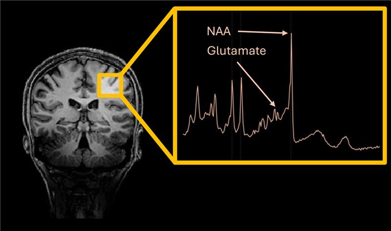
MR Spectroscopy (MRS)#
Quantification of concentration of various metabolites (chemical compounds)
Each metabolite has a distinct spectral (frequency-domain) signature based on its chemical structure
Introduction#
This example demonstrates the processing of MR spectra acquired from the human motor cortex using Osprey, a standalone tool for processing and quantification of magnetic resonance spectroscopy (MRS) data.
Citation and Resources:#
Tools included in this workflow#
Osprey:
Oeltzschner, G., Zöllner, H. J., Hui, S. C. N., Mikkelsen, M., Saleh, M. G., Tapper, S., & Edden, R. A. E. (2020). Osprey: Open-source processing, reconstruction & estimation of magnetic resonance spectroscopy data. Journal of Neuroscience Methods, 343, 108827. https://doi.org/10.1016/j.jneumeth.2020.108827
Python:
Python Software Foundation. (2023). Python (Version 3.11.6) [Software]. Available at https://www.python.org/
Dataset#
Collected at UQ as part of the BeLong study
T1 weighted MP2RAGE at 3T (healthy control)
SEMI-LASER MRS at 3T (healthy control)
Oz, G., & Tkáč, I. (2011). Short-echo, single-shot, full-intensity proton magnetic resonance spectroscopy for neurochemical profiling at 4 T: validation in the cerebellum and brainstem. Magn Reson Med, 65(4), 901-910. https://doi.org/10.1002/mrm.22708
Deelchand, D. K., Berrington, A., Noeske, R., Joers, J. M., Arani, A., Gillen, J., Schär, M., Nielsen, J. F., Peltier, S., Seraji-Bozorgzad, N., Landheer, K., Juchem, C., Soher, B. J., Noll, D. C., Kantarci, K., Ratai, E. M., Mareci, T. H., Barker, P. B., & Öz, G. (2021). Across-vendor standardization of semi-LASER for single-voxel MRS at 3T. NMR Biomed, 34(5), e4218. https://doi.org/10.1002/nbm.4218
The basis file used in this example is a placeholder, the SLaser basis set used in the acquisition (Eftekhari, Z., Shaw, T., Deelchand, D., Marjańska, M., Bogner, W., & Barth, M. (2025). Reliability and Reproducibility of Metabolite Quantification Using 1H MRS in the Human Brain at 3 T and 7 T. NMR in biomedicine, 38, e70087. https://doi.org/10.1002/nbm.70087) is not shareable at the moment.
Osprey input#
Description |
Filename |
|---|---|
Raw metabolite data |
mrs/…svs_slaser_dkd_ul.dat |
Water reference data |
mrs/…svs_slaser_dkd_ul_wref.dat |
T1-weighted anatomical image |
anat/…acq-MP2RAGE_T1w.nii |
JSON file configuring the pipeline. See Osprey’s documentation for more details |
osprey-job.json |
A BASIS file containing simulated model spectra for known metabolites. Used by LCModel to fit data. |
set.BASIS |
Osprey output#
Description |
Filename |
|---|---|
MRS voxel aligned with the anatomy |
osprey-output/VoxelMasks/…svs_slaser_dkd_ul_space-scanner_mask.nii |
MRS voxel segmentation masks (GM, WM, CSF) |
osprey-output/SegMaps/…svs_slaser_dkd_ul_space-scanner_Voxel-1_label-CSF.nii |
Results of spectral fitting (from LCmodel) |
osprey-output/LCMOutput/ |
Summary of results from different steps of the pipeline. It includes some QC metrics |
osprey-output/Reports/sub-002-report.html |
Tables with concentration values for metabolites using different references |
osprey-output/QuantifyResults/ |
Load software tools and import python libraries#
import module
await module.load('osprey/2.9.0')
await module.list()
['osprey/2.9.0']
%%capture
!pip install nibabel numpy pandas
import os
from pathlib import Path
import shutil
from IPython.display import Image as ipython_image, display, HTML
from PIL import Image, ImageDraw, ImageFont
from ipyniivue import NiiVue
import nibabel as nib
import numpy as np
import ipywidgets as widgets
import pandas as pd
import matplotlib.pyplot as plt
import json
import subprocess
Set up Osprey Job configuration#
Download and prepare data
Set up paths to the relevant MRS/MRI files
Set up the configuration JSON file
Check that all specified paths exist
NOTE: For a more detailed explanation of all the configuration options see Osprey’s documentation
%%bash
echo "Downloading data"
osf -p 3a2ws fetch osfstorage/osprey.zip ./data_osprey/osprey.zip
echo "Unzipping data"
unzip ./data_osprey/osprey.zip -d ./data_osprey/
Downloading data
Unzipping data
Archive:  ./data_osprey/osprey.zip
   creating: ./data_osprey/sub-002/ses-01/
   creating: ./data_osprey/sub-002/ses-01/anat/
  inflating: ./data_osprey/sub-002/ses-01/anat/sub-002_ses-01_acq-MP2RAGE_desc-defaced_T1w.nii
   creating: ./data_osprey/sub-002/ses-01/mrs/
  inflating: ./data_osprey/sub-002/ses-01/mrs/meas_MID00104_FID130221_svs_slaser_dkd_ul_wref.dat
  inflating: ./data_osprey/sub-002/ses-01/mrs/meas_MID00103_FID130220_svs_slaser_dkd_ul.dat
100%|██████████| 150M/150M [00:16<00:00, 9.38Mbytes/s]
# Get path to Osprey executable.
osprey_path = subprocess.check_output("which ospreyCMD", shell=True, text=True).strip()

# Extract container base and image path.
container_base = os.path.dirname(osprey_path)
container_id = os.path.basename(container_base)
simg_path = os.path.join(container_base, f"{container_id}.simg")

# Construct the basis set path (from inside the container).
basis_path = os.path.join(
    simg_path,
    "opt/basissets/3T/siemens/unedited/slaser/30"
)

# Osprey will try to convert this .mat basis file into a .BASIS type
# file. It will try to write the new .BASIS file into the same folder
# where the .mat basis file is. Thus, the .mat basis file needs to be
# copied into a writeable location.
!cp {basis_path}/basis_siemens_slaser30.mat ./data_osprey/basis_siemens_slaser30.mat
base_path = os.getcwd()
data_path = f'{base_path}/data_osprey'
output_path = f'{base_path}/osprey-output'
basis_set = f'{data_path}/basis_siemens_slaser30.mat'
job_path = f'{base_path}/osprey-job.json'

sub = 'sub-002'
ses = 'ses-01'

# Metabolite data.
files = [
    f'{data_path}/{sub}/{ses}/mrs/meas_MID00103_FID130220_svs_slaser_dkd_ul.dat'
]
# Water reference data.
files_ref = [
    f'{data_path}/{sub}/{ses}/mrs/meas_MID00104_FID130221_svs_slaser_dkd_ul_wref.dat'
]
# T1.
files_nii = [
    f'{data_path}/{sub}/{ses}/anat/{sub}_{ses}_acq-MP2RAGE_desc-defaced_T1w.nii'
]
mrs_options = {
    'seqType': 'unedited',
    'editTarget': ['none'],
    'dataScenario': 'invivo',
    'outputFolder': [output_path],
    'SpecReg': 'RobSpecReg',
    'SubSpecAlignment': 'none',
    'EECraw': '1',
    'ECCmm': '1',
    'method': 'LCModel',
    'saveLCM': '1',
    'savejMRUI': '0',
    'saveVendor': '1',
    'saveNII': '1',
    'savePDF': '0',
    'includeMetabs': ['default'],
    'style': 'Separate',
    'range': ['0.5', '4.2'],
    'rangeWater': ['2.0', '7.4'],
    'bLineKnotSpace': '5',
    'fitMM': '1',
    'basisSet': basis_set,
    'files': files,
    'files_ref': files_ref,
    'files_nii': files_nii
}

with open(job_path, 'w') as f:
    json.dump(mrs_options, f)
check_paths = [data_path, output_path, basis_set, job_path]
check_paths = check_paths + files + files_ref + files_nii

# Create the results directory if it doesn't exist yet
os.makedirs(output_path, exist_ok=True)

any_warning = False
for pth in check_paths:
    pth_exists = Path(pth).exists()
    print(f"{'✅' if pth_exists else '❌'}  '{pth}'")
✅  '/home/jovyan/Git_repositories/example-notebooks/books/spectroscopy/data_osprey'
✅  '/home/jovyan/Git_repositories/example-notebooks/books/spectroscopy/osprey-output'
✅  '/home/jovyan/Git_repositories/example-notebooks/books/spectroscopy/data_osprey/basis_siemens_slaser30.mat'
✅  '/home/jovyan/Git_repositories/example-notebooks/books/spectroscopy/osprey-job.json'
✅  '/home/jovyan/Git_repositories/example-notebooks/books/spectroscopy/data_osprey/sub-002/ses-01/mrs/meas_MID00103_FID130220_svs_slaser_dkd_ul.dat'
✅  '/home/jovyan/Git_repositories/example-notebooks/books/spectroscopy/data_osprey/sub-002/ses-01/mrs/meas_MID00104_FID130221_svs_slaser_dkd_ul_wref.dat'
✅  '/home/jovyan/Git_repositories/example-notebooks/books/spectroscopy/data_osprey/sub-002/ses-01/anat/sub-002_ses-01_acq-MP2RAGE_desc-defaced_T1w.nii'
Run Osprey processing#
The following command runs the Oprey CLI software with specifications from the job file defined above.
!ospreyCMD {job_path}
------------------------------------------
Setting up environment variables
---
LD_LIBRARY_PATH is .:/opt/MCR/R2023a//runtime/glnxa64:/opt/MCR/R2023a//bin/glnxa64:/opt/MCR/R2023a//sys/os/glnxa64:/opt/MCR/R2023a//sys/opengl/lib/glnxa64
Spectral fitting parameters will not be saved (default). Please indicate otherwise in the csv-file or the GUI
/home/jovyan/Git_repositories/example-notebooks/books/spectroscopy/osprey-job.json
Timestamp October 30, 2025 00:07:41 Osprey 2.9.0
Timestamp October 30, 2025 00:07:41 Osprey 2.9.0  OspreyLoad
Loading raw data from dataset   1 out of   1 total datasets...
Software version: VD (!?)
Reader version: 1496740353 (UTC: 06-Jun-2017 09:12:33)
Scan 1/2, read all mdhs:
    35.3 MB read in    0 s
Scan 2/2, read all mdhs:
    83.9 MB read in    0 s

ans =

     0

multi RAID file detected.
Software version: VD (!?)
Reader version: 1496740353 (UTC: 06-Jun-2017 09:12:33)
Scan 1/2, read all mdhs:
    35.3 MB read in    0 s
Scan 2/2, read all mdhs:
    19.0 MB read in    0 s

ans =

     0

multi RAID file detected.

... done.
 Elapsed time 15.933984 seconds
Timestamp October 30, 2025 00:07:57 Osprey 2.9.0  OspreyProcess
Processing data from dataset   1 out of   1 total datasets...

... done.
 Elapsed time 57.194783 seconds
Writing table to file = /home/jovyan/Git_repositories/example-notebooks/books/spectroscopy/osprey-output/QM_processed_spectra.tsv
Writing table to file = /home/jovyan/Git_repositories/example-notebooks/books/spectroscopy/osprey-output/QM_processed_spectra.json
Timestamp October 30, 2025 00:08:56 Osprey 2.9.0  OspreyFit
Fitting metabolite spectra from dataset   1 out of   1 total datasets...

... done.
 Elapsed time 4.912133 seconds

... done.
 Elapsed time 4.912133 seconds
Writing table to file = /home/jovyan/Git_repositories/example-notebooks/books/spectroscopy/osprey-output/QM_processed_spectra.tsv
Writing table to file = /home/jovyan/Git_repositories/example-notebooks/books/spectroscopy/osprey-output/QM_processed_spectra.json
Timestamp October 30, 2025 00:09:07 Osprey 2.9.0  OspreyCoreg
Coregistering voxel from dataset   1 out of   1 total datasets...

... done.
 Elapsed time 6.378909 seconds
Timestamp October 30, 2025 00:09:14 Osprey 2.9.0  OspreySeg

Segmenting structural image from dataset   1 out of   1 total datasets...


------------------------------------------------------------------------
30-Oct-2025 00:09:22 - Running job #1
------------------------------------------------------------------------
30-Oct-2025 00:09:22 - Running 'Segment'

SPM12: spm_preproc_run (v7670)                     00:09:22 - 30/10/2025
========================================================================
Segment /home/jovyan/Git_repositories/example-notebooks/books/spectroscopy/data_osprey/sub-002/ses-01/anat/sub-002_ses-01_acq-MP2RAGE_desc-defaced_T1w.nii,1
Completed                               :          00:12:55 - 30/10/2025
30-Oct-2025 00:12:55 - Done    'Segment'
30-Oct-2025 00:12:55 - Done


------------------------------------------------------------------------
30-Oct-2025 00:12:59 - Running job #1
------------------------------------------------------------------------
30-Oct-2025 00:12:59 - Running 'Normalise: Write'
30-Oct-2025 00:13:10 - Done    'Normalise: Write'
30-Oct-2025 00:13:10 - Done


------------------------------------------------------------------------
30-Oct-2025 00:13:14 - Running job #1
------------------------------------------------------------------------
30-Oct-2025 00:13:14 - Running 'Image Calculator'

SPM12: spm_imcalc (v6961)                          00:13:14 - 30/10/2025
========================================================================
ImCalc Image: /home/jovyan/Git_repositories/example-notebooks/books/spectroscopy/osprey-output/VoxelMasks/MID00103_FID130220_svs_slaser_dkd_ul_space-spm152_mask_VoxelOverlap.nii
30-Oct-2025 00:13:15 - Done    'Image Calculator'
30-Oct-2025 00:13:15 - Done


... done.
 Elapsed time 234.532095 seconds
Writing table to file = /home/jovyan/Git_repositories/example-notebooks/books/spectroscopy/osprey-output/SegMaps/TissueFractions_Voxel_1.tsv
Writing table to file = /home/jovyan/Git_repositories/example-notebooks/books/spectroscopy/osprey-output/SegMaps/TissueFractions_Voxel_1.json
Timestamp October 30, 2025 00:13:16 Osprey 2.9.0  OspreyQuantify

Quantifying dataset   1 out of   1 total datasets...

... done.
 Elapsed time 0.064912 seconds
Writing table to file = /home/jovyan/Git_repositories/example-notebooks/books/spectroscopy/osprey-output/QuantifyResults/A_amplMets_Voxel_1_Basis_1.tsv
Writing table to file = /home/jovyan/Git_repositories/example-notebooks/books/spectroscopy/osprey-output/QuantifyResults/A_amplMets_Voxel_1_Basis_1.json
Writing table to file = /home/jovyan/Git_repositories/example-notebooks/books/spectroscopy/osprey-output/QuantifyResults/A_tCr_Voxel_1_Basis_1.tsv
Writing table to file = /home/jovyan/Git_repositories/example-notebooks/books/spectroscopy/osprey-output/QuantifyResults/A_tCr_Voxel_1_Basis_1.json
Writing table to file = /home/jovyan/Git_repositories/example-notebooks/books/spectroscopy/osprey-output/QuantifyResults/A_rawWaterScaled_Voxel_1_Basis_1.tsv
Writing table to file = /home/jovyan/Git_repositories/example-notebooks/books/spectroscopy/osprey-output/QuantifyResults/A_rawWaterScaled_Voxel_1_Basis_1.json
Writing table to file = /home/jovyan/Git_repositories/example-notebooks/books/spectroscopy/osprey-output/QuantifyResults/A_CSFWaterScaled_Voxel_1_Basis_1.tsv
Writing table to file = /home/jovyan/Git_repositories/example-notebooks/books/spectroscopy/osprey-output/QuantifyResults/A_CSFWaterScaled_Voxel_1_Basis_1.json
Writing table to file = /home/jovyan/Git_repositories/example-notebooks/books/spectroscopy/osprey-output/QuantifyResults/A_TissCorrWaterScaled_Voxel_1_Basis_1.tsv
Writing table to file = /home/jovyan/Git_repositories/example-notebooks/books/spectroscopy/osprey-output/QuantifyResults/A_TissCorrWaterScaled_Voxel_1_Basis_1.json
Writing table to file = /home/jovyan/Git_repositories/example-notebooks/books/spectroscopy/osprey-output/QuantifyResults/A_AlphaCorrWaterScaled_Voxel_1_Basis_1.tsv
Writing table to file = /home/jovyan/Git_repositories/example-notebooks/books/spectroscopy/osprey-output/QuantifyResults/A_AlphaCorrWaterScaled_Voxel_1_Basis_1.json
Writing table to file = /home/jovyan/Git_repositories/example-notebooks/books/spectroscopy/osprey-output/QuantifyResults/A_AlphaCorrWaterScaledGroupNormed_Voxel_1_Basis_1.tsv
Writing table to file = /home/jovyan/Git_repositories/example-notebooks/books/spectroscopy/osprey-output/QuantifyResults/A_AlphaCorrWaterScaledGroupNormed_Voxel_1_Basis_1.json
Writing table to file = /home/jovyan/Git_repositories/example-notebooks/books/spectroscopy/osprey-output/QuantifyResults/A_CRLB_Voxel_1_Basis_1.tsv
Writing table to file = /home/jovyan/Git_repositories/example-notebooks/books/spectroscopy/osprey-output/QuantifyResults/A_CRLB_Voxel_1_Basis_1.json
Writing table to file = /home/jovyan/Git_repositories/example-notebooks/books/spectroscopy/osprey-output/QuantifyResults/A_h2oarea_Voxel_1_Basis_1.tsv
Writing table to file = /home/jovyan/Git_repositories/example-notebooks/books/spectroscopy/osprey-output/QuantifyResults/A_h2oarea_Voxel_1_Basis_1.json
Timestamp October 30, 2025 00:13:18 Osprey 2.9.0  OspreyOverview

Gathering spectra from subspectrum 1 out of 2 total subspectra..Gathering spectra from subspectrum 1 out of 2 total subspectra..Gathering spectra from subspectrum 2 out of 2 total subspectra...
... done.
Gathering fit models from fit 1 out of 1 total fits.Gathering fit models from fit 1 out of 1 total fits...
... done.
Interpolating fit models from fit 1 out of 1 total fits.Interpolating fit models from fit 1 out of 1 total fits...
... done.

Scaling data from dataset 1 out of 1 total datasets.Scaling data from dataset 1 out of 1 total datasets.Scaling data from dataset 1 out of 1 total datasets...
... done.
Writing table to file = /home/jovyan/Git_repositories/example-notebooks/books/spectroscopy/osprey-output/subject_names_and_excluded.tsv
Writing table to file = /home/jovyan/Git_repositories/example-notebooks/books/spectroscopy/osprey-output/subject_names_and_excluded.json
... done.
 Elapsed time 0.289561 seconds
Runtime Breakdown................
OspreyLoad runtime: 15.933984 seconds
OspreyProcess runtime: 57.194783 seconds
OspreyFit runtime: 4.912133 seconds
	OspreyFit metab runtime: 4.912133 seconds
OspreyCoreg runtime: 6.378909 seconds
OspreySeg runtime: 234.532095 seconds
OspreyOverview runtime: 0.289561 seconds
Full Osprey runtime: 319.306377 seconds
Results#
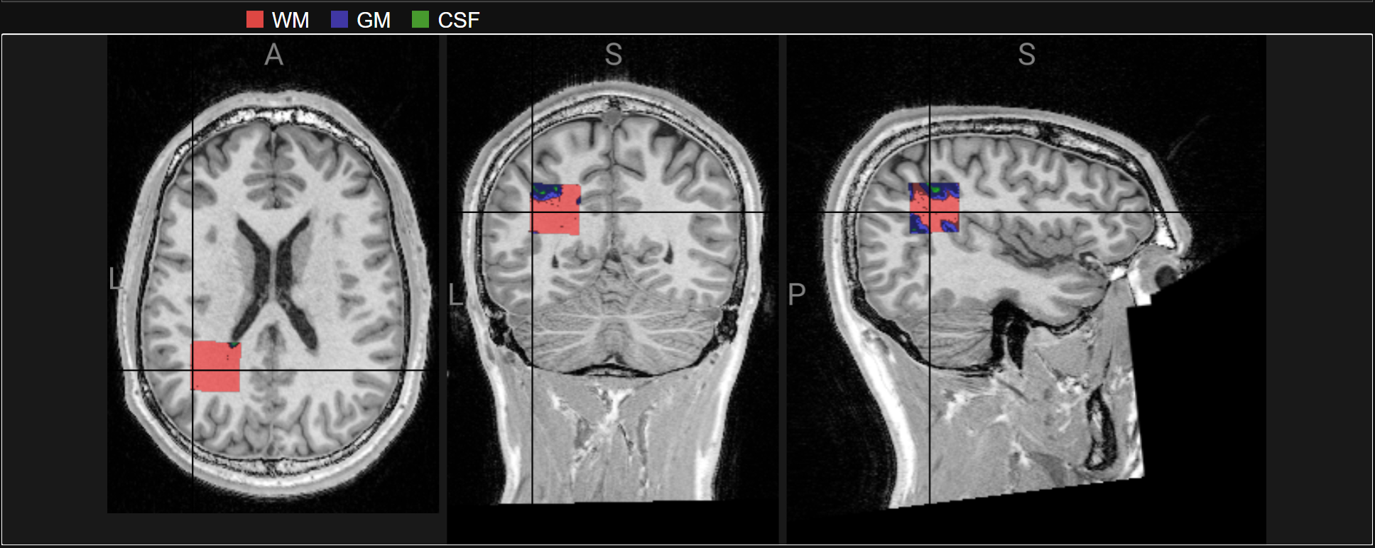
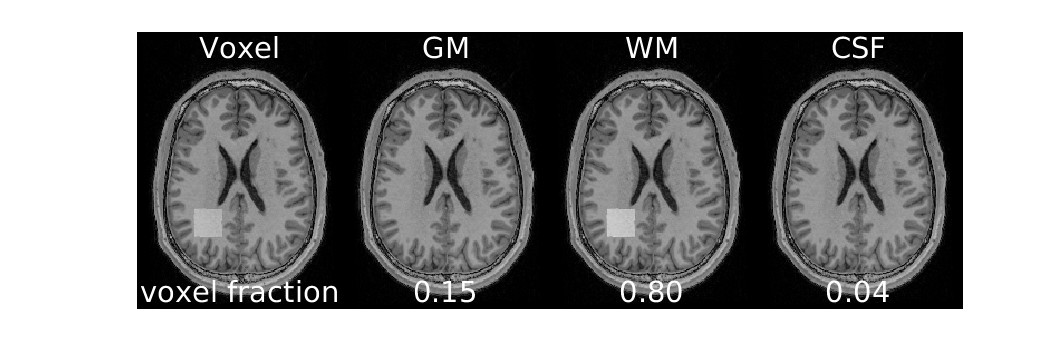
T1s with the MRS voxel aligned#
Osprey performs alignment with T1
Osprey also performs segmentation to determine the proportion of tissue types within the voxel (for WM and CSF correction)
# Prepare the main viewer withot the 3D render.
nv = NiiVue(
    height=600,
    multiplanar_layout="ROW",
    multiplanar_show_render=False,
    multiplanar_pad_pixels=10,
    is_ruler=False,
    is_colorbar=False,
    is_orient_cube=False,
    is_radiological_convention=False,
    back_color=(0.1,0.1,0.1,1.0),
    crosshair_color=[0,0,0,1]
)

# Robust intensity window (ignore zeros and outliers)
t1 = nib.load(files_nii[0]).get_fdata()
vals = t1[t1 > 0]
vmin, vmax = np.percentile(vals, [0.5, 99.5]) if vals.size else (None, None)

# T1 with contrast adjusted.
nv.add_volume({
    "path": files_nii[0],
    "name": "native",
    "opacity": 1.0,
    "colormap": "gray",
    "cal_min": float(vmin) if vmin is not None else None,
    "cal_max": float(vmax) if vmax is not None else None,
    "ignore_zero_voxels": True,
})

# WM segmentation.
nv.add_volume({
    "path": f'{output_path}/SegMaps/meas_MID00103_FID130220_svs_slaser_dkd_ul_space-scanner_Voxel-1_label-WM.nii.gz',
    "name": "wm",
    "opacity": 0.5,
    "colormap": "red",
    "ignore_zero_voxels": True,
})

# GM segmentation.
nv.add_volume({
    "path": f'{output_path}/SegMaps/meas_MID00103_FID130220_svs_slaser_dkd_ul_space-scanner_Voxel-1_label-GM.nii.gz',
    "name": "gm",
    "opacity": 0.5,
    "colormap": "blue",
    "ignore_zero_voxels": True,
})

# CSF segmentation.
nv.add_volume({
    "path": f'{output_path}/SegMaps/meas_MID00103_FID130220_svs_slaser_dkd_ul_space-scanner_Voxel-1_label-CSF.nii.gz',
    "name": "csf",
    "opacity": 0.5,
    "colormap": "green",
    "ignore_zero_voxels": True,
})

# Add legend (in HTML so we can style).
fontsize = 25
entry_sep = 25
text_sep = 10
cube_size = 20
capt = widgets.HTML(
    f"<div style='font:{fontsize}px sans-serif; margin-left:285px;'>"
    f"<div style='display:inline-block; margin-right:{entry_sep}px;'>"
    f"<span style='display:inline-block; width:{cube_size}px; height:{cube_size}px; background-color:#de4743; margin-right:{text_sep}px;'></span>WM"
    "</div>"
    f"<div style='display:inline-block; margin-right:{entry_sep}px;'>"
    f"<span style='display:inline-block; width:{cube_size}px; height:{cube_size}px; background-color:#4037a4; margin-right:{text_sep}px;'></span>GM"
    "</div>"
    f"<div style='display:inline-block; margin-right:{entry_sep}px;'>"
    f"<span style='display:inline-block; width:{cube_size}px; height:{cube_size}px; background-color:#479a2e; margin-right:{text_sep}px;'></span>CSF"
    "</div>"
    "</div>"
)
# Put the legend above the NiiVue viewer.
panel = widgets.VBox([capt, nv])

display(panel)
display(ipython_image(url='https://raw.githubusercontent.com/neurodesk/example-notebooks/refs/heads/main/books/images/osprey-notebook.png'))
display(ipython_image(filename=f"{output_path}/Reports/reportFigures/sub-002/sub-002_seg_svs_space-scanner_mask.jpg"))
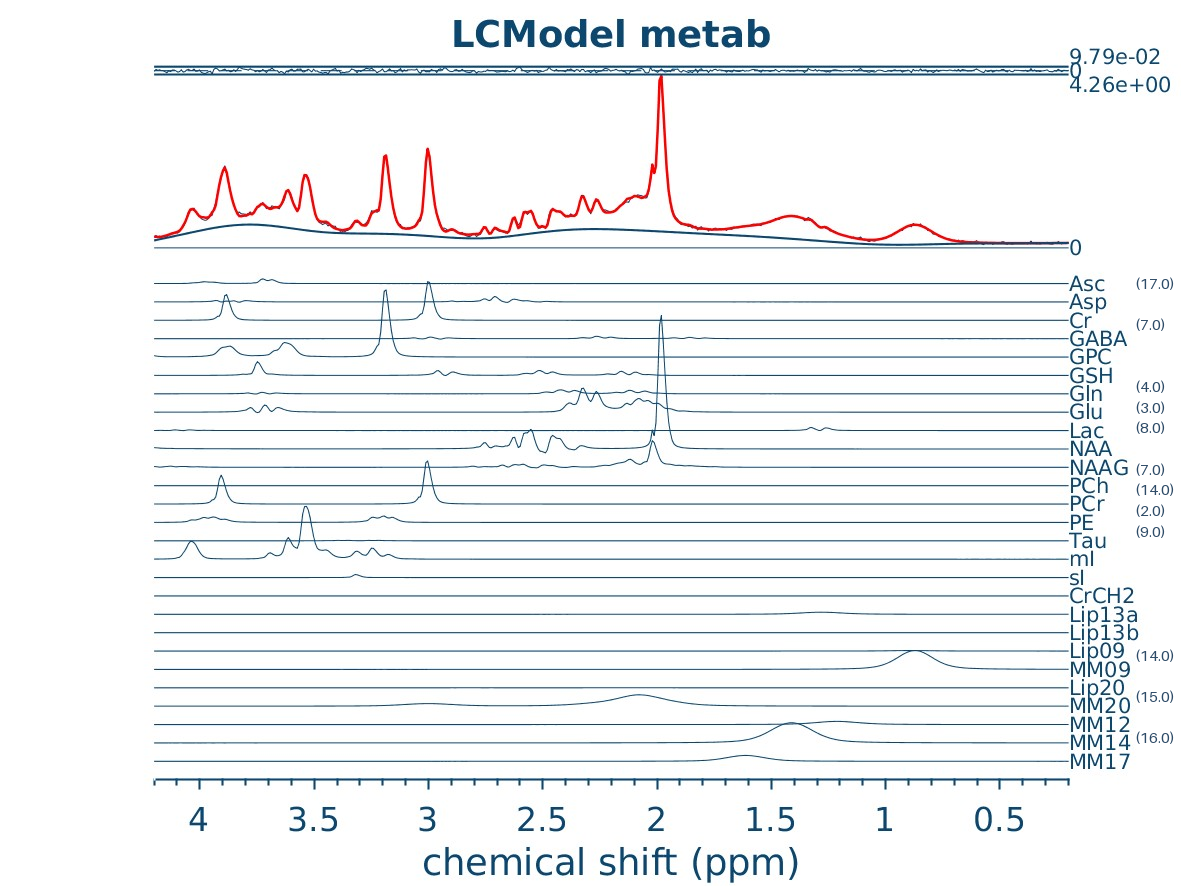
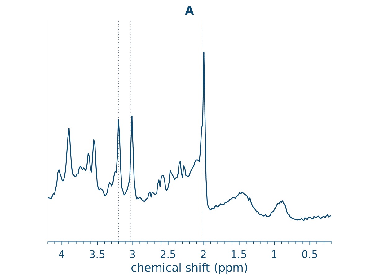
Spectral modelling#
Osprey runs LCModel for spectral fitting
crlb_threshold = 20

# Make sure to only include the metabolites in the LCmodel plot.
metabolites = [
    'Asp', 'Asc', 'Cr', 'GABA', 'Gln', 'Glu', 'GPC', 'GSH', 'Lac',
    'PCr', 'PE', 'NAA', 'NAAG', 'Tau', 'CrCH2', 'Lip13a', 'Lip13b',
    'Lip09', 'MM09', 'Lip20', 'MM20', 'MM12', 'MM14', 'MM17'
]

# crlbs = pd.read_csv(f'{output_path}/QuantifyResults/A_CRLB_Voxel_1_Basis_1.tsv', delimiter='\t')[metabolites]
crlbs = pd.read_csv(f'{output_path}/QuantifyResults/A_CRLB_Voxel_1_Basis_1.tsv', delimiter='\t')[metabolites]
crlb_dict = crlbs.iloc[0, :].to_dict()

# Osprey fitting results image.
img_path = f"{output_path}/Reports/reportFigures/sub-002/sub-002_metab_A_model.jpg"
img = Image.open(img_path)

# Draw CRLBs on top of the image.
draw = ImageDraw.Draw(img)
font = ImageFont.load_default(size=15)

x, y = 1135, 253
for met, crlb in crlb_dict.items():
    y += 20.67  # shift down for next line
    # Only show
    if crlb < crlb_threshold:
        draw.text((x, y), f"({crlb:.1f})", fill="#2e4b67", font=font)

display(img)
# Centered title
display(HTML("<h2 style='text-align: center;'>Averaged Spectra</h2>"))

# Image (keeps default alignment unless styled otherwise)
display(ipython_image(filename=f"{output_path}/Reports/reportFigures/sub-002/sub-002_metab_A.jpg"))
Averaged Spectra
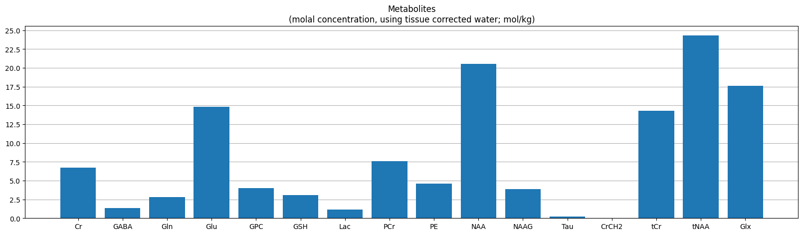
Metabolite concetrations#
Osprey calculates metabolite concentrations relative to different references
metabolites = ['Cr', 'GABA', 'Gln', 'Glu', 'GPC', 'GSH', 'Lac', 'PCr', 'PE', 'NAA', 'NAAG', 'Tau', 'CrCH2', 'tCr', 'tNAA', 'Glx']

def plot_metabolites(data, figsize=(20, 5), label='(raw values in arbitrary units)', ytick_step=0.2):
    fig = plt.figure(figsize=figsize)
    ax = fig.add_subplot()
    ax.bar(height=data.values[0], x=data.columns, zorder=2)
    ax.set_title(f'Metabolites\n{label}')

    ylims = ax.get_ylim()
    yticks = np.arange(ylims[0], ylims[1], ytick_step)
    ax.set_yticks(yticks)

    ax.grid(axis='y', zorder=1)
met_data = pd.read_csv(f'{output_path}/QuantifyResults/A_tCr_Voxel_1_Basis_1.tsv', delimiter='\t')
plot_metabolites(met_data[metabolites], label='(ratio of tCR)')

met_data = pd.read_csv(f'{output_path}/QuantifyResults/A_TissCorrWaterScaled_Voxel_1_Basis_1.tsv', delimiter='\t')
plot_metabolites(met_data[metabolites], label='(molal concentration, using tissue corrected water; mol/kg)', ytick_step=2.5)
Dependencies in Jupyter/Python#
Using the package watermark to document system environment and software versions used in this notebook
%load_ext watermark

%watermark
%watermark --iversions
Last updated: 2025-10-30T00:13:39.768416+00:00

Python implementation: CPython
Python version       : 3.11.6
IPython version      : 8.16.1

Compiler    : GCC 12.3.0
OS          : Linux
Release     : 5.4.0-204-generic
Machine     : x86_64
Processor   : x86_64
CPU cores   : 32
Architecture: 64bit

PIL       : 10.3.0
matplotlib: 3.8.4
numpy     : 2.2.6
ipywidgets: 8.1.2
nibabel   : 5.2.1
json      : 2.0.9
ipyniivue : 2.3.2
IPython   : 8.16.1
pandas    : 2.3.3