Run this notebook
Date: 1 May 2025
License:
Note: If this notebook uses neuroimaging tools from Neurocontainers, those tools retain their original licenses. Please see Neurodesk citation guidelines for details.
Citation and Resources:
Tools included in this workflow
AFNI
Cox RW (1996). AFNI: software for analysis and visualization of functional magnetic resonance neuroimages. Comput Biomed Res 29(3):162-173. doi:10
.1006 /cbmr .1996 .0014 RW Cox, JS Hyde (1997). Software tools for analysis and visualization of FMRI Data. NMR in Biomedicine, 10: 171-178. https://
pubmed .ncbi .nlm .nih .gov /9430344/
Educational Resources
Andy’s Brain Book:
This AFNI example is based on the AFNI Tutorial: Statistics and Modeling from Andy’s Brain Book (Jahn, 2022. doi:10
.5281 /zenodo .5879293)
Dataset
Flanker Dataset from OpenNeuro:
Kelly AMC and Uddin LQ and Biswal BB and Castellanos FX and Milham MP (2018). Flanker task (event-related). OpenNeuro Dataset ds000102. [Dataset] doi: null
Kelly AM, Uddin LQ, Biswal BB, Castellanos FX, Milham MP. Competition between functional brain networks mediates behavioral variability. Neuroimage. 2008 Jan 1;39(1):527-37. doi: Kelly et al. (2008). Epub 2007 Aug 23. PMID: 17919929.
Mennes, M., Kelly, C., Zuo, X.N., Di Martino, A., Biswal, B.B., Castellanos, F.X., Milham, M.P. (2010). Inter-individual differences in resting-state functional connectivity predict task-induced BOLD activity. Neuroimage, 50(4):1690-701. doi: Mennes et al. (2010). Epub 2010 Jan 15. Erratum in: Neuroimage. 2011 Mar 1;55(1):434
Mennes, M., Zuo, X.N., Kelly, C., Di Martino, A., Zang, Y.F., Biswal, B., Castellanos, F.X., Milham, M.P. (2011). Linking inter-individual differences in neural activation and behavior to intrinsic brain dynamics. Neuroimage, 54(4):2950-9. doi: Mennes et al. (2011)
Introduction
First Level fMRI Analysis with AFNI: Preprocessing and GLM
Building on the preprocessing pipeline introduced in the Preprocessing with AFNI notebook, this notebook extends the workflow to include a General Linear Model (GLM) for modelling task-related brain activity. The GLM is a core method in fMRI analysis that estimates the brain’s response to experimental conditions by fitting a model to the observed signal. We again work with subject sub-08 from the DS000102 Flanker task dataset.
By the end of this notebook, you will be able to:
Add a GLM (regress block) to an
afni_proc.pypreprocessing pipelineUnderstand how timing files and HRF modelling work in AFNI
Inspect and interpret the GLM design matrix
Use AFNI’s automated quality control outputs to assess preprocessing success
Visualise first-level statistical maps using Nilearn
Load AFNI
import module
await module.load('afni/25.2.03')
await module.list()['afni/25.2.03']Import Python Modules
%%capture
!pip install nibabel==5.3.3 numpy==2.3.5 nilearn==0.13.1 scipy==1.16.3
import os
import nibabel as nib
import numpy as np
import matplotlib.pyplot as plt
import matplotlib
from IPython.display import display, Image
from nilearn import plotting
from nilearn.image import math_img
from scipy.stats import tData download
PATTERN = "sub-08"%%bash -s "$PATTERN"
set -euo pipefail
# Retry transient network failures, then fail the cell instead of continuing without data.
retry() { for i in 1 2 3 4 5; do "$@" && return 0; echo "Attempt $i failed: $*" >&2; [ "$i" -lt 5 ] && sleep $((i * 15)); done; return 1; }
PATTERN=$1
[ -d ds000102 ] || retry datalad install https://github.com/OpenNeuroDatasets/ds000102.git
cd ds000102 && retry datalad get $PATTERN[INFO] Attempting a clone into /home/jovyan/workspace/books/examples/functional_imaging/ds000102
[INFO] Attempting to clone from https://github.com/OpenNeuroDatasets/ds000102.git to /home/jovyan/workspace/books/examples/functional_imaging/ds000102
[INFO] Start enumerating objects
[INFO] Start counting objects
[INFO] Start compressing objects
[INFO] Start receiving objects
[INFO] Start resolving deltas
[INFO] Completed clone attempts for Dataset(/home/jovyan/workspace/books/examples/functional_imaging/ds000102)
[INFO] Remote origin not usable by git-annex; setting annex-ignore
[INFO] https://github.com/OpenNeuroDatasets/ds000102.git/config download failed: Not Found
[INFO] access to 1 dataset sibling s3-PRIVATE not auto-enabled, enable with:
| datalad siblings -d "/home/jovyan/workspace/books/examples/functional_imaging/ds000102" enable -s s3-PRIVATE
install(ok): /home/jovyan/workspace/books/examples/functional_imaging/ds000102 (dataset)
get(ok): sub-08/anat/sub-08_T1w.nii.gz (file) [from s3-PUBLIC...]
get(ok): sub-08/func/sub-08_task-flanker_run-1_bold.nii.gz (file) [from s3-PUBLIC...]
get(ok): sub-08/func/sub-08_task-flanker_run-2_bold.nii.gz (file) [from s3-PUBLIC...]
get(ok): sub-08 (directory)
action summary:
  get (ok: 4)
The data is structured in BIDS format:
!tree -L 4 ds000102Create timing files
To model brain activity during different conditions of the Flanker task, we first need to create timing files based on the experimental events. These files capture when each trial occurred, how long it lasted, and whether any parametric modulation should be applied. This information is stored in each subject’s events.tsv file. We will extract the relevant details - condition name, onset, and duration - and convert them into AFNI’s timing file format. For each condition (congruent and incongruent), we will generate timing files for both runs, then combine them into condition-specific .1D files. These timing files will later be used in the GLM (general linear model) to estimate brain responses to each condition.
To automate this process, we will download a Bash script called make_Timings.sh from Andy’s AFNI_Scripts repository. This script should be placed in the experimental folder containing the subject directories (in our case, the ds000102/ folder).
![ -f ds000102/make_Timings.sh ] || wget -O ds000102/make_Timings.sh https://raw.githubusercontent.com/andrewjahn/AFNI_Scripts/master/make_Timings.sh--2026-10-08 16:01:17-- https://raw.githubusercontent.com/andrewjahn/AFNI_Scripts/master/make_Timings.sh
Resolving raw.githubusercontent.com (raw.githubusercontent.com)... 185.199.111.133, 185.199.110.133, 185.199.109.133, ...
Connecting to raw.githubusercontent.com (raw.githubusercontent.com)|185.199.111.133|:443... connected.
HTTP request sent, awaiting response... 200 OK
Length: 953 [text/plain]
Saving to: ‘ds000102/make_Timings.sh’
ds000102/make_Timin 100%[===================>] 953 --.-KB/s in 0s
2026-10-08 16:01:17 (77.3 MB/s) - ‘ds000102/make_Timings.sh’ saved [953/953]
Once the script is downloaded into the ds000102/ folder, we can execute it directly from the notebook. The command below does three things:
cd ds000102changes into the experimental directory that contains the subject folders.chmod +x make_Timings.shmakes the script executable.bash make_Timings.shruns the script.
After running this command, you should see new timing files (e.g., congruent.1D, incongruent.1D) inside each subject’s func/ directory. These files are now ready to be used in the first-level GLM analysis.
!cd ds000102 && chmod +x make_Timings.sh && bash make_Timings.shCheck the output:
!cat ds000102/sub-08/func/incongruent.1D0 10 20 52 88 130 144 174 248 260 274
0 10 52 64 88 150 164 174 196 232 260
Running Preprocessing and First Level Analysis for sub-08
All of the preprocessing steps (from setup through scaling) for subject sub-08 were introduced and explained in the example notebook about Preprocessing with AFNI- which is highly inspired by Andy’s Brain Book’s excellent AFNI tutorial.
There, it is covered how to use afni_proc.py to generate an automated pipeline, and how to interpret each preprocessing block. In this section, we extend that workflow by adding a regress block to model task-related brain activity using a general linear model (GLM):
➡️
setup ➡️ tcat ➡️ tshift ➡️ align ➡️ tlrc ➡️ volreg ➡️ blur ➡️ mask ➡️ scale ➡️ regress ➡️ 🧠✅ outputs: preprocessed EPI, tSNR maps, motion parameters, fitted time series, beta weights, and statistical maps — estimated via 3dREMLfit with HRF modeling (GAM), motion and outlier censoring, and symbolic GLTs.
!afni_proc.py                                                                            \
    -subj_id                 sub_08                                                      \
    -script                  proc.sub_08                                                 \
    -scr_overwrite                                                                       \
    -out_dir                 ./afni_pro_glm/sub_08.results                               \
    -blocks                  tshift align tlrc volreg blur mask scale                    \
                             regress                                                     \
    -copy_anat               ./ds000102/sub-08/anat/sub-08_T1w.nii.gz                    \
    -dsets                                                                               \
                             ./ds000102/sub-08/func/sub-08_task-flanker_run-1_bold.nii.gz \
                             ./ds000102/sub-08/func/sub-08_task-flanker_run-2_bold.nii.gz \
    -radial_correlate_blocks tcat volreg                                                 \
    -tcat_remove_first_trs   0                                                            \
    -align_unifize_epi       local                                                        \
    -align_opts_aea          -cost lpc+ZZ                                                \
                             -giant_move                                                 \
                             -check_flip                                                  \
    -tlrc_base               MNI152_2009_template_SSW.nii.gz                             \
    -tlrc_opts_at            -init_xform AUTO_CENTER                                     \
    -volreg_align_to         MIN_OUTLIER                                                 \
    -volreg_align_e2a                                                                    \
    -volreg_tlrc_warp                                                                    \
    -volreg_compute_tsnr     yes                                                         \
    -volreg_warp_dxyz        3.0                                                         \
    -mask_epi_anat           yes                                                         \
    -blur_size               5.0                                                         \
    -regress_stim_times      ./ds000102/sub-08/func/congruent.1D                         \
                             ./ds000102/sub-08/func/incongruent.1D                       \
    -regress_stim_labels     congruent incongruent                                       \
    -regress_basis           GAM                                                         \
    -regress_censor_motion   0.3                                                         \
    -regress_censor_outliers 0.05                                                        \
    -regress_motion_per_run                                                              \
    -regress_opts_3dD        -jobs 8                                                     \
                             -gltsym 'SYM: incongruent -congruent'                       \
                             -glt_label 1 incongruent-congruent                          \
                             -gltsym 'SYM: congruent -incongruent'                       \
                             -glt_label 2 congruent-incongruent                          \
    -regress_reml_exec                                                                   \
    -regress_compute_fitts                                                                \
    -regress_make_ideal_sum  sum_ideal.1D                                                \
    -regress_est_blur_epits                                                              \
    -regress_est_blur_errts                                                              \
    -regress_run_clustsim    no
-- applying input view as +orig
-- template = 'MNI152_2009_template_SSW.nii.gz', exists = 1
-- have APQC atlas APQC_atlas_MNI_2009c_asym.nii.gz
-- will use min outlier volume as motion base
-- including default: -find_var_line_blocks tcat
-- tcat: reps is now 146
++ updating polort to 2, from run len 292.0 s
-- volreg: using base dset vr_base_min_outlier+orig
++ volreg: applying volreg/epi2anat/tlrc xforms to isotropic 3 mm tlrc voxels
-- applying anat warps to 1 dataset(s): sub-08_T1w
++ mask: using epi_anat mask in place of EPI one
-- masking: group anat = 'MNI152_2009_template_SSW.nii.gz', exists = 1
-- have 2 ROI dict entries ...
++ will compute regress TSNR stats for dsets: brain, MNI_2009c_asym
-- using default: will not apply EPI Automask
(see 'MASKING NOTE' from the -help for details)
--> script is file: proc.sub_08
to execute via tcsh:
tcsh -xef proc.sub_08 |& tee output.proc.sub_08
to execute via bash:
tcsh -xef proc.sub_08 2>&1 | tee output.proc.sub_08
Below is a brief explanation of the key options added to afni_proc.py:
-blocks ... tshift ... regress: Adds slice timing correction (tshift) and the GLM regression step (regress) to the processing pipeline. Slice timing correction accounts for the fact that different brain slices are acquired at slightly different times within each TR. The regress block estimates condition-specific brain activity using a GLM.
-regress_stim_times: Points to the timing .1D files (e.g., congruent.1D, incongruent.1D) we created earlier. These specify when each condition occurred during the experiment.
-regress_stim_labels: Assigns labels to the timing files. These labels are used internally in AFNI (and in our symbolic GLTs) to refer to each condition.
-regress_basis GAM: Applies the canonical hemodynamic response function (HRF) using a Gamma function, which models the typical shape of neural activation over time in response to a stimulus.
-regress_censor_motion 0.3: Censors TRs where estimated head motion exceeds 0.3mm framewise displacement, preventing motion artifacts from contaminating the GLM.
-regress_censor_outliers 0.05: Additionally censors TRs where more than 5% of brain voxels are statistical outliers — providing an extra layer of data quality control beyond motion alone.
-regress_motion_per_run: Estimates separate motion parameter regressors for each run, which is more appropriate than a single set when data comes from multiple runs.
-regress_opts_3dD: Passes additional options to the 3dDeconvolve command that runs the regression. In this case:
-gltsym 'SYM: incongruent -congruent': Defines a contrast comparing incongruent > congruent.-gltsym 'SYM: congruent -incongruent': Defines the reverse contrast, congruent > incongruent.-glt_label: Assigns human-readable labels to each contrast.-jobs 8: Specifies using 8 CPU threads for faster computation.-regress_reml_exec: Tells AFNI to run 3dREMLfit, which uses a more sophisticated model of temporal autocorrelation. This is typically more accurate than the default 3dDeconvolve and recommended for group-level analysis later.
-regress_compute_fitts: Saves the full fitted (modeled) timeseries to disk, useful for visualizing model fit and computing residuals.
-regress_est_blur_epits / -regress_est_blur_errts: Estimates the effective spatial smoothness of the data from both the preprocessed EPI timeseries and the residuals after regression. These estimates are used later for cluster-level thresholding at the group level.
-regress_run_clustsim no: Disables real-time cluster-level threshold simulations, since we’re not doing single-subject inference.
Running the Preprocessing and GLM Script
With the script proc.sub_08 prepared, we’re ready to run it. This will carry out all preprocessing steps followed by the GLM analysis and and logs the full output to output.proc.sub_08, allowing to review everything that happened during processing:
! tcsh -xef proc.sub_08 |& tee output.proc.sub_08Results: Examining the output
Let’s take a look at the results directory. Files containing the "pb" string are the preprocessed functional images at each step of the pipeline, while those with "T1w" refer to the preprocessed anatomical images. Additional auxiliary functional images are generated to assist with specific preprocessing steps, and auxiliary text files store information such as transformation matrices and motion parameters.
The file named stats.sub_08+tlrc contains results from the traditional 3dDeconvolve analysis, whereas stats.sub_08_REML+tlrc contains results from the 3dREMLfit approach, which accounts for temporal autocorrelation.
You’ll also see several files beginning with "X", such as X.xmat.1D, which represent components of the design matrix used in the regression analysis.
AFNI also automatically creates a quality control directory named QC_sub_08.
!ls ./afni_pro_glm/sub_08.results@epi_review.sub_08
@ss_review_basic
@ss_review_driver
@ss_review_driver_commands
MNI152_2009_template_SSW.nii.gz
QC_sub_08
ROI_import_MNI_2009c_asym+tlrc.BRIK
ROI_import_MNI_2009c_asym+tlrc.HEAD
ROI_import_MNI_2009c_asym_resam+tlrc.BRIK
ROI_import_MNI_2009c_asym_resam+tlrc.HEAD
TSNR.sub_08+tlrc.BRIK
TSNR.sub_08+tlrc.HEAD
TSNR.vreg.r01.sub_08+tlrc.BRIK
TSNR.vreg.r01.sub_08+tlrc.HEAD
X.jpg
X.nocensor.xmat.1D
X.stim.xmat.1D
X.xmat.1D
__tt_lr_flipcosts.1D
__tt_lr_noflipcosts.1D
aea_checkflip_results.txt
all_runs.sub_08+tlrc.BRIK
all_runs.sub_08+tlrc.HEAD
anat_final.sub_08+tlrc.BRIK
anat_final.sub_08+tlrc.HEAD
anat_w_skull_warped+tlrc.BRIK
anat_w_skull_warped+tlrc.HEAD
blur.epits.1D
blur.err_reml.1D
blur.errts.1D
blur_est.sub_08.1D
censor_sub_08_combined_2.1D
corr_brain+tlrc.BRIK
corr_brain+tlrc.HEAD
dfile.r01.1D
dfile.r02.1D
dfile_rall.1D
errts.sub_08+tlrc.BRIK
errts.sub_08+tlrc.HEAD
errts.sub_08_REML+tlrc.BRIK
errts.sub_08_REML+tlrc.HEAD
files_ACF
final_epi_vr_base_min_outlier+tlrc.BRIK
final_epi_vr_base_min_outlier+tlrc.HEAD
fitts.sub_08+tlrc.BRIK
fitts.sub_08+tlrc.HEAD
fitts.sub_08_REML+tlrc.BRIK
fitts.sub_08_REML+tlrc.HEAD
full_mask.sub_08+tlrc.BRIK
full_mask.sub_08+tlrc.HEAD
ideal_congruent.1D
ideal_incongruent.1D
mask_anat.sub_08+tlrc.BRIK
mask_anat.sub_08+tlrc.HEAD
mask_epi_anat.sub_08+tlrc.BRIK
mask_epi_anat.sub_08+tlrc.HEAD
mask_epi_extents+tlrc.BRIK
mask_epi_extents+tlrc.HEAD
mask_group+tlrc.BRIK
mask_group+tlrc.HEAD
mat.basewarp.aff12.1D
mat.r01.vr.aff12.1D
mat.r01.warp.aff12.1D
mat.r02.vr.aff12.1D
mat.r02.warp.aff12.1D
mean.errts.1D
mean.errts.unit.1D
mot_demean.r01.1D
mot_demean.r02.1D
motion_demean.1D
motion_deriv.1D
motion_sub_08_CENSORTR.txt
motion_sub_08_censor.1D
motion_sub_08_enorm.1D
out.4095_all.txt
out.4095_warn.txt
out.allcostX.txt
out.ap_uvars.json
out.ap_uvars.txt
out.cormat_warn.txt
out.df_info.txt
out.gcor.1D
out.keep_trs_rall.txt
out.mask_ae_dice.txt
out.mask_ae_overlap.txt
out.mask_at_dice.txt
out.min_outlier.txt
out.pre_ss_warn.txt
out.ss_review.sub_08.txt
out.ss_review_uvars.json
out.vlines.pb00.tcat.txt
outcount.r01.1D
outcount.r02.1D
outcount_rall.1D
outcount_sub_08_censor.1D
pb00.sub_08.r01.tcat+orig.BRIK
pb00.sub_08.r01.tcat+orig.HEAD
pb00.sub_08.r02.tcat+orig.BRIK
pb00.sub_08.r02.tcat+orig.HEAD
pb01.sub_08.r01.tshift+orig.BRIK
pb01.sub_08.r01.tshift+orig.HEAD
pb01.sub_08.r02.tshift+orig.BRIK
pb01.sub_08.r02.tshift+orig.HEAD
pb02.sub_08.r01.volreg+tlrc.BRIK
pb02.sub_08.r01.volreg+tlrc.HEAD
pb02.sub_08.r02.volreg+tlrc.BRIK
pb02.sub_08.r02.volreg+tlrc.HEAD
pb03.sub_08.r01.blur+tlrc.BRIK
pb03.sub_08.r01.blur+tlrc.HEAD
pb03.sub_08.r02.blur+tlrc.BRIK
pb03.sub_08.r02.blur+tlrc.HEAD
pb04.sub_08.r01.scale+tlrc.BRIK
pb04.sub_08.r01.scale+tlrc.HEAD
pb04.sub_08.r02.scale+tlrc.BRIK
pb04.sub_08.r02.scale+tlrc.HEAD
pre.sub-08_T1w_ns+orig.BRIK
pre.sub-08_T1w_ns+orig.HEAD
pre.sub-08_T1w_ns_WarpDrive.log
radcor.pb00.tcat
radcor.pb02.volreg
run_graphview_errts.tcsh
run_graphview_pbrun.tcsh
run_instacorr_errts.tcsh
run_instacorr_pbrun.tcsh
run_qc_00_vorig_EPI.tcsh
run_qc_01_vorig_anat.tcsh
run_qc_03_ve2a_epi2anat.tcsh
run_qc_04_va2t_anat2temp.tcsh
run_qc_05_va2t_mask2final.tcsh
run_qc_06_vstat_Full_Fstat.tcsh
run_qc_07_vstat_congruent_0_Coef.tcsh
run_qc_08_vstat_incongruent_0_Coef.tcsh
run_qc_09_vstat_incongruent-congruent_0_Coef.tcsh
run_qc_10_vstat_congruent-incongruent_0_Coef.tcsh
run_qc_17_regr_corr_errts.tcsh
run_qc_18_regr_tsnr_vreg.tcsh
run_qc_19_regr_tsnr_fin.tcsh
run_qc_21_radcor_rc_tcat_r01.tcsh
run_qc_21_radcor_rc_tcat_r02.tcsh
run_qc_22_radcor_rc_volreg_r01.tcsh
run_qc_22_radcor_rc_volreg_r02.tcsh
run_qc_28_warns_flip_0.tcsh
run_qc_28_warns_flip_1.tcsh
stats.REML_cmd
stats.sub_08+tlrc.BRIK
stats.sub_08+tlrc.HEAD
stats.sub_08_REML+tlrc.BRIK
stats.sub_08_REML+tlrc.HEAD
stats.sub_08_REMLvar+tlrc.BRIK
stats.sub_08_REMLvar+tlrc.HEAD
stimuli
sub-08_T1w+orig.BRIK
sub-08_T1w+orig.HEAD
sub-08_T1w_al_junk+orig.BRIK
sub-08_T1w_al_junk+orig.HEAD
sub-08_T1w_al_junk_mat.aff12.1D
sub-08_T1w_flip__al_junk_mat.aff12.1D
sub-08_T1w_flip_al_junk+orig.BRIK
sub-08_T1w_flip_al_junk+orig.HEAD
sub-08_T1w_ns+orig.BRIK
sub-08_T1w_ns+orig.HEAD
sub-08_T1w_ns+tlrc.BRIK
sub-08_T1w_ns+tlrc.HEAD
sub-08_T1w_ns.Xaff12.1D
sub-08_T1w_ns.Xat.1D
sub-08_T1w_ns.maskwarp.Xat.1D
sub-08_T1w_ns_shft.1D
sub-08_T1w_unflipped+orig.BRIK
sub-08_T1w_unflipped+orig.HEAD
sub-08_T1w_unflipped_ns+orig.BRIK
sub-08_T1w_unflipped_ns+orig.HEAD
sub-08_T1w_unflipped_ns_al_junk_wtal+orig.BRIK
sub-08_T1w_unflipped_ns_al_junk_wtal+orig.HEAD
sum_ideal.1D
tsnr_stats_regress
vlines.pb00.tcat
volumized+tlrc.BRIK
volumized+tlrc.HEAD
vr_base_min_outlier+orig.BRIK
vr_base_min_outlier+orig.HEAD
vr_base_min_outlier_unif+orig.BRIK
vr_base_min_outlier_unif+orig.HEAD
vr_base_min_outlier_unif_ts_ns+orig.BRIK
vr_base_min_outlier_unif_ts_ns+orig.HEAD
vr_base_min_outlier_unif_ts_ns_wt+orig.BRIK
vr_base_min_outlier_unif_ts_ns_wt+orig.HEAD
warp.anat.Xat.1D
Design Matrix
Let’s visualize the graphical representation of the design matrix to check the experimental design setup. The image shows how each condition (stimulus) is modeled across the time series. The "X" files contain important information about how the stimuli, motion parameters, and other regressors are combined into the matrix for the GLM analysis.
In this case, the design matrix includes the following regressors in order:
The first 6 regressors (
Run#1Pol#0toRun#2Pol#2) are drift (polynomial) terms used to model low-frequency signal fluctuations separately for each run.The next 2 regressors (
congruent#0andincongruent#0) correspond to the task-related conditions and model stimulus events across both runs.The final 6 regressors (
mot_demean[0]#0tomot_demean[5]#0) represent motion parameters for the entire session, capturing estimated head movement in 3 translational and 3 rotational directions.
display(Image(filename='./afni_pro_glm/sub_08.results/X.jpg', width=700))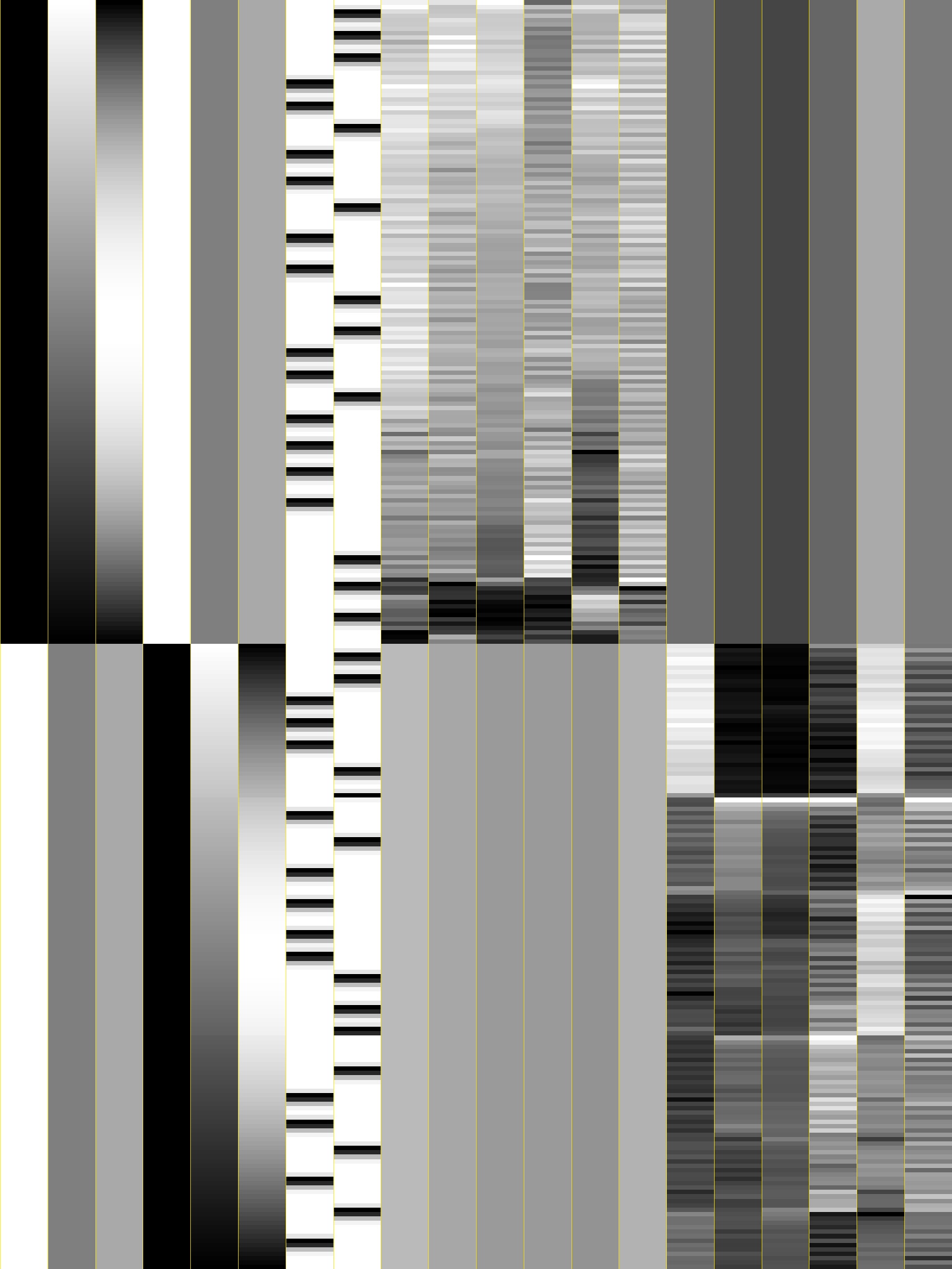
To view the names of the individual regressors in the design matrix, you can run the following command. This will list the labels in the same order they appear in the matrix, helping you verify which columns correspond to drift terms, task conditions, and motion parameters.
!1d_tool.py -infile ./afni_pro_glm/sub_08.results/X.xmat.1D -show_labels++ labels are: ['Run#1Pol#0', 'Run#1Pol#1', 'Run#1Pol#2', 'Run#2Pol#0', 'Run#2Pol#1', 'Run#2Pol#2', 'congruent#0', 'incongruent#0', 'mot_demean_r01[0]#0', 'mot_demean_r01[1]#0', 'mot_demean_r01[2]#0', 'mot_demean_r01[3]#0', 'mot_demean_r01[4]#0', 'mot_demean_r01[5]#0', 'mot_demean_r02[0]#0', 'mot_demean_r02[1]#0', 'mot_demean_r02[2]#0', 'mot_demean_r02[3]#0', 'mot_demean_r02[4]#0', 'mot_demean_r02[5]#0']
In addition to this, you’ll also see a visualization of the design matrix using the file X.xmat.1D below. This provides another way to examine the structure of the GLM model, showing when each regressor is active across the time series. Make sure the design matrix looks reasonable.
# Load the design matrix
xmat = np.loadtxt('./afni_pro_glm/sub_08.results/X.xmat.1D')

# Set up number of regressors and colors
n_regressors = xmat.shape[1]
colors = matplotlib.colormaps.get_cmap('tab20').resampled(n_regressors)

# Plot each regressor in its own row with a distinct color
fig, axes = plt.subplots(nrows=n_regressors, ncols=1, figsize=(12, n_regressors * 0.8), sharex=True)

for i in range(n_regressors):
    ax = axes[i]
    ax.plot(xmat[:, i], color=colors(i))
    ax.set_yticks([])
    ax.set_ylabel(f'{i+1}', rotation=0, fontsize=8, labelpad=15)
    ax.spines['top'].set_visible(False)
    ax.spines['right'].set_visible(False)
    ax.spines['left'].set_visible(False)

axes[-1].set_xlabel('Time points (TRs)', fontsize=10)
plt.suptitle('AFNI Design Matrix: X.xmat.1D', fontsize=14)
plt.tight_layout(rect=[0, 0, 1, 0.96])
plt.show()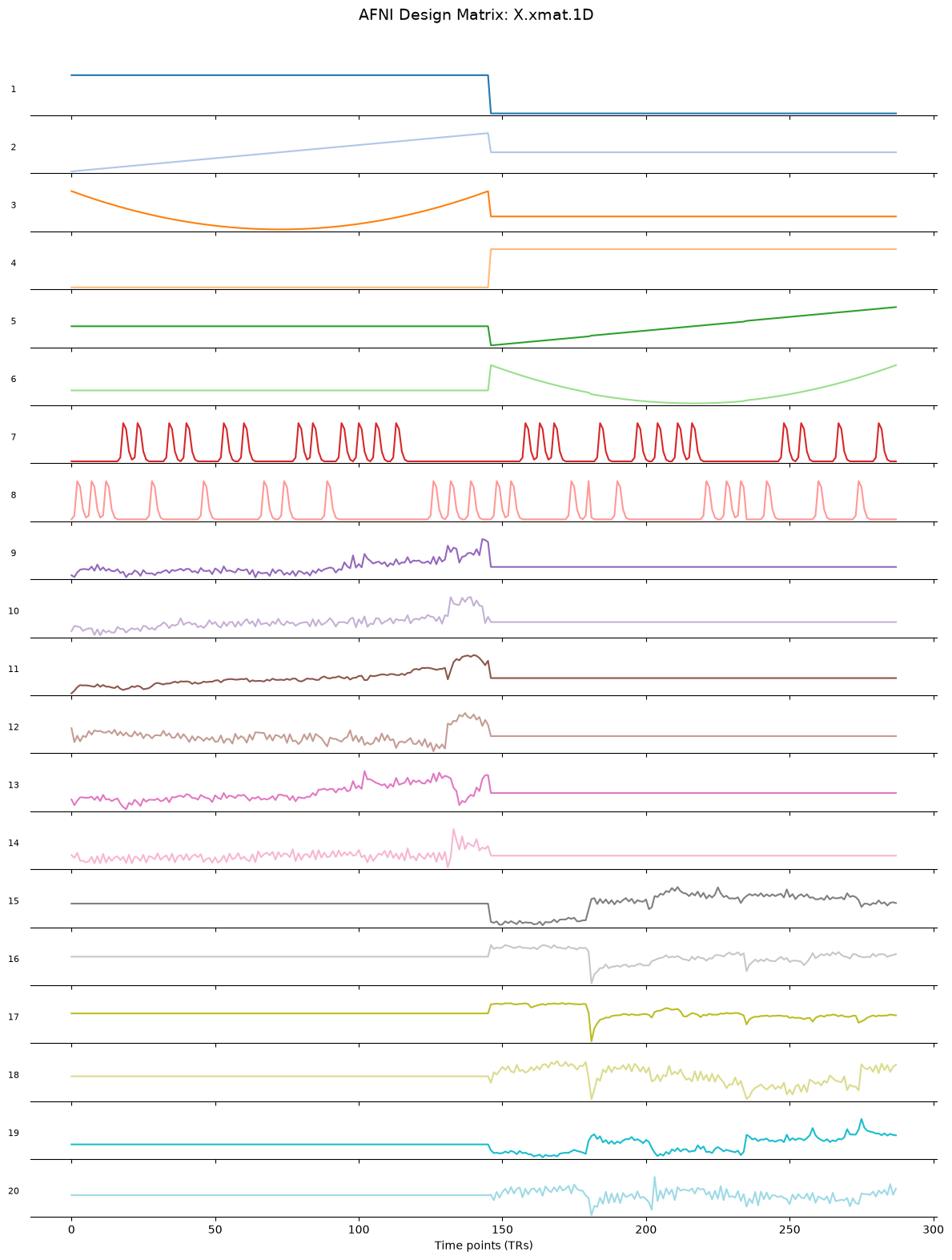
Quality Check
AFNI automatically generates a quality control directory named QC_sub_08, which contains images and summary metrics for each preprocessing and GLM step such as motion estimates, outlier fractions and EPI-to-anatomical alignment. These quality control plots are stored in the media/ subfolder and can be displayed within the notebook to visually inspect the success of each step.
The show_qc_image() function can be used to display quality control images directly within the notebook. It takes the image filename and an optional title to present relevant QC plots inline.
We display two types of QC images: registration checks (EPI-to-anatomical and anatomical-to-template alignment) and statistical maps (F-statistic and beta coefficients for each condition and contrast).
def show_qc_image(filename, title=None):
    from IPython.display import Image, display
    if title:
        print(f'\n📊 {title}')
    display(Image(filename=filename))
show_qc_image('./afni_pro_glm/sub_08.results/QC_sub_08/media/qc_03_ve2a_epi2anat.axi.jpg', 'EPI to Anatomical Alignment')
📊 EPI to Anatomical Alignment

show_qc_image('./afni_pro_glm/sub_08.results/QC_sub_08/media/qc_04_va2t_anat2temp.sag.jpg', 'Anatomical to MNI template Alignment')
📊 Anatomical to MNI template Alignment

show_qc_image('./afni_pro_glm/sub_08.results/QC_sub_08/media/qc_06_vstat_Full_Fstat.axi.jpg', 'Full F_stat (stats.sub_08_REML)')
📊 Full F_stat (stats.sub_08_REML)

show_qc_image('./afni_pro_glm/sub_08.results/QC_sub_08/media/qc_07_vstat_congruent_0_Coef.sag.jpg',
              'Congruent — Beta Coefficient')
📊 Congruent — Beta Coefficient

show_qc_image('./afni_pro_glm/sub_08.results/QC_sub_08/media/qc_08_vstat_incongruent_0_Coef.sag.jpg',
              'Incongruent — Beta Coefficient')
📊 Incongruent — Beta Coefficient

show_qc_image('./afni_pro_glm/sub_08.results/QC_sub_08/media/qc_09_vstat_incongruent-congruent_0_Coef.sag.jpg',
              'Incongruent > Congruent — Beta Coefficient')
📊 Incongruent > Congruent — Beta Coefficient

show_qc_image('./afni_pro_glm/sub_08.results/QC_sub_08/media/qc_10_vstat_congruent-incongruent_0_Coef.sag.jpg',
              'Congruent > Incongruent — Beta Coefficient')
📊 Congruent > Incongruent — Beta Coefficient

Statistical Maps with Nilearn
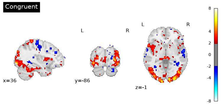
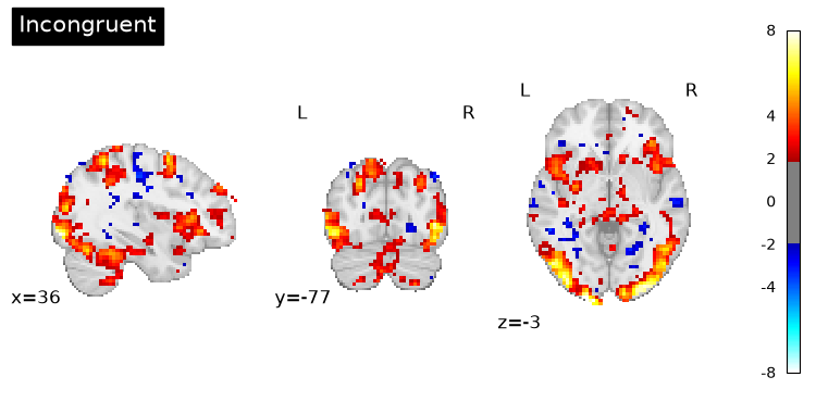
The AFNI QC images above show the results using AFNI’s own display settings. Here, we recreate these contrast maps using Nilearn, which allows more control over thresholding, colormaps, and display — and demonstrates how to work with AFNI’s sub-brick structure programmatically.
First, we convert the stats.sub_08_REML file to NIfTI format using 3dAFNItoNIFTI, and inspect the sub-brick structure of the stats dataset using 3dinfo to identify which indices correspond to our conditions and contrasts of interest.
!3dAFNItoNIFTI -prefix ./afni_pro_glm/sub_08.results/stats.sub_08_REML+tlrc.nii.gz ./afni_pro_glm/sub_08.results/stats.sub_08_REML+tlrc++ 3dAFNItoNIFTI: AFNI version=AFNI_25.2.03 (Jul 4 2025) [64-bit]
!3dinfo -verb ./afni_pro_glm/sub_08.results/stats.sub_08+tlrc.HEAD++ 3dinfo: AFNI version=AFNI_25.2.03 (Jul 4 2025) [64-bit]
Dataset File: stats.sub_08+tlrc
Identifier Code: XYZ_7YGJtrtCtvndgHrBmtAZHA Creation Date: Thu Oct 8 16:07:33 2026
Template Space: MNI_2009c_asym
Dataset Type: Func-Bucket (-fbuc)
Byte Order: LSB_FIRST [this CPU native = LSB_FIRST]
Storage Mode: BRIK
Storage Space: 16,187,392 (16 million) bytes
Geometry String: "MATRIX(-3,0,0,94.5,0,-3,0,130.5,0,0,3,-76.5):64,76,64"
Data Axes Tilt: Plumb
Data Axes Orientation:
first (x) = Left-to-Right
second (y) = Posterior-to-Anterior
third (z) = Inferior-to-Superior [-orient LPI]
R-to-L extent: -94.500 [R] -to- 94.500 [L] -step- 3.000 mm [ 64 voxels]
A-to-P extent: -94.500 [A] -to- 130.500 [P] -step- 3.000 mm [ 76 voxels]
I-to-S extent: -76.500 [I] -to- 112.500 [S] -step- 3.000 mm [ 64 voxels]
Number of values stored at each pixel = 13
-- At sub-brick #0 'Full_Fstat' datum type is float: 0 to 61.0312
statcode = fift; statpar = 2 268
-- At sub-brick #1 'congruent#0_Coef' datum type is float: -17.2177 to 14.3244
-- At sub-brick #2 'congruent#0_Tstat' datum type is float: -4.61816 to 7.86733
statcode = fitt; statpar = 268
-- At sub-brick #3 'congruent_Fstat' datum type is float: 0 to 61.8948
statcode = fift; statpar = 1 268
-- At sub-brick #4 'incongruent#0_Coef' datum type is float: -15.1565 to 14.6077
-- At sub-brick #5 'incongruent#0_Tstat' datum type is float: -5.25655 to 9.84963
statcode = fitt; statpar = 268
-- At sub-brick #6 'incongruent_Fstat' datum type is float: 0 to 97.0152
statcode = fift; statpar = 1 268
-- At sub-brick #7 'incongruent-congruent_GLT#0_Coef' datum type is float: -16.799 to 16.6239
-- At sub-brick #8 'incongruent-congruent_GLT#0_Tstat' datum type is float: -4.70007 to 5.90507
statcode = fitt; statpar = 268
-- At sub-brick #9 'incongruent-congruent_GLT_Fstat' datum type is float: 0 to 34.8699
statcode = fift; statpar = 1 268
-- At sub-brick #10 'congruent-incongruent_GLT#0_Coef' datum type is float: -16.6239 to 16.799
-- At sub-brick #11 'congruent-incongruent_GLT#0_Tstat' datum type is float: -5.90507 to 4.70007
statcode = fitt; statpar = 268
-- At sub-brick #12 'congruent-incongruent_GLT_Fstat' datum type is float: 0 to 34.8699
statcode = fift; statpar = 1 268
----- HISTORY -----
[jovyan@c4ed8d6c5732: Thu Oct 8 16:07:33 2026] {AFNI_25.2.03:linux_ubuntu_24_64} 3dDeconvolve -input pb04.sub_08.r01.scale+tlrc.HEAD pb04.sub_08.r02.scale+tlrc.HEAD -censor censor_sub_08_combined_2.1D -ortvec mot_demean.r01.1D mot_demean_r01 -ortvec mot_demean.r02.1D mot_demean_r02 -polort 2 -num_stimts 2 -stim_times 1 stimuli/congruent.1D GAM -stim_label 1 congruent -stim_times 2 stimuli/incongruent.1D GAM -stim_label 2 incongruent -jobs 8 -gltsym 'SYM: incongruent -congruent' -glt_label 1 incongruent-congruent -gltsym 'SYM: congruent -incongruent' -glt_label 2 congruent-incongruent -fout -tout -x1D X.xmat.1D -xjpeg X.jpg -x1D_uncensored X.nocensor.xmat.1D -errts errts.sub_08 -bucket stats.sub_08
[jovyan@c4ed8d6c5732: Thu Oct 8 16:07:33 2026] Output prefix: stats.sub_08
🧠 Summary of Regressors and Contrasts
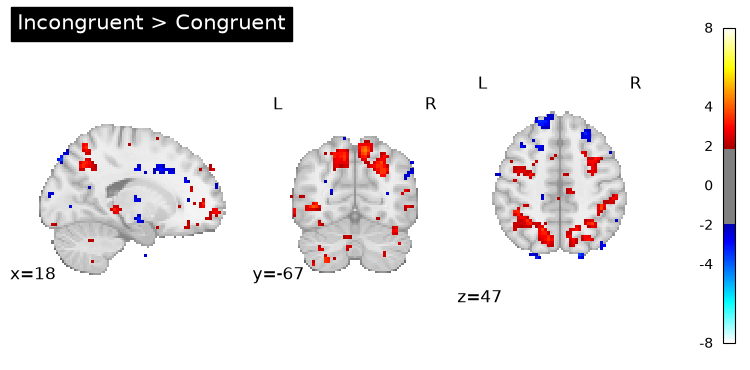
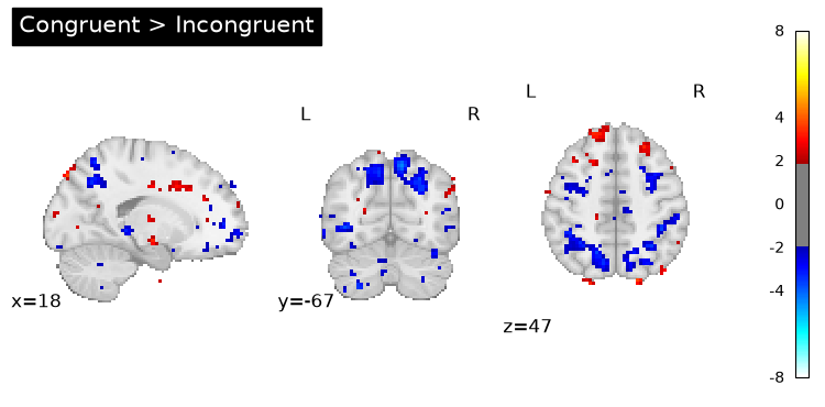
The following table provides key information from the 3dinfo output of the stats.sub_08_REML dataset. It includes the regressors (conditions) and contrasts, as well as their associated T-statistics. These values will be visualized as T-stat maps using Nilearn to examine the statistical significance of the task-related effects.
| Sub-brick | Label | Meaning |
|---|---|---|
| #1 | congruent#0_Coef | Beta weight (coefficient) for congruent trials |
| #4 | incongruent#0_Coef | Beta weight (coefficient) for incongruent trials |
| #7 | incongruent-congruent_GLT#0_Coef | Beta weight (coefficient) for the contrast between incongruent and congruent trials |
| #10 | congruent-incongruent_GLT#0_Coef | Beta weight (coefficient) for the contrast between congruent and incongruent trials |
| #2 | congruent#0_Tstat | T-statistic for congruent trials |
| #5 | incongruent#0_Tstat | T-statistic for incongruent trials |
| #8 | incongruent-congruent_GLT#0_Tstat | T-statistic for incongruent > congruent |
| #11 | congruent-incongruent_GLT#0_Tstat | T-statistic for congruent > incongruent |
%%bash
# Convert brain mask from AFNI format (.HEAD/.BRIK) to NIfTI for use with nilearn
3dAFNItoNIFTI -prefix ./afni_pro_glm/sub_08.results/full_mask.sub_08+tlrc.nii.gz \
    ./afni_pro_glm/sub_08.results/full_mask.sub_08+tlrc
++ 3dAFNItoNIFTI: AFNI version=AFNI_25.2.03 (Jul 4 2025) [64-bit]
# Degrees of freedom (statpar) - from the GLM output
df = 278
# Calculate the critical t-value for two-tailed p=0.05
alpha = 0.05
critical_t_value = t.ppf(1 - alpha/2, df)
print(f"Critical t-value for p=0.05 and df={df}: {np.round(critical_t_value,3)}")

# Load the REML statistics file containing all contrasts as sub-bricks
img = nib.load('./afni_pro_glm/sub_08.results/stats.sub_08_REML+tlrc.nii.gz')
data = img.get_fdata()
affine = img.affine

# Extract t-statistic maps for each contrast (sub-brick indices from 3dinfo)
tstat_congruent = data[:, :, :, 0, 2]            # sub-brick #2
tstat_incongruent = data[:, :, :, 0, 5]          # sub-brick #5
tstat_incongruent_gt_congruent = data[:, :, :, 0, 8]   # sub-brick #8
tstat_congruent_gt_incongruent = data[:, :, :, 0, 11]  # sub-brick #11

# Make NIfTI images
tstat_congruent_img = nib.Nifti1Image(tstat_congruent, affine)
tstat_incongruent_img = nib.Nifti1Image(tstat_incongruent, affine)
tstat_contrast1_img = nib.Nifti1Image(tstat_incongruent_gt_congruent, affine)
tstat_contrast2_img = nib.Nifti1Image(tstat_congruent_gt_incongruent, affine)

# Apply brain mask to restrict display to brain voxels only
brain_mask = nib.load('./afni_pro_glm/sub_08.results/full_mask.sub_08+tlrc.nii.gz')

def apply_brain_mask(stat_img, mask_img):
    return math_img("img * mask", img=stat_img, mask=mask_img)

tstat_congruent_img = apply_brain_mask(tstat_congruent_img, brain_mask)
tstat_incongruent_img = apply_brain_mask(tstat_incongruent_img, brain_mask)
tstat_contrast1_img = apply_brain_mask(tstat_contrast1_img, brain_mask)
tstat_contrast2_img = apply_brain_mask(tstat_contrast2_img, brain_mask)

# Plot each contrast thresholded at the critical t-value
plotting_config = {
    "display_mode": "ortho",
    "draw_cross": False,
    "vmax": 8,
    "cmap": "cold_hot",  # blue = negative, red = positive
    "colorbar": True,
}

for img, title in [
    (tstat_congruent_img, "Congruent"),
    (tstat_incongruent_img, "Incongruent"),
    (tstat_contrast1_img, "Incongruent > Congruent"),
    (tstat_contrast2_img, "Congruent > Incongruent"),
]:
    plotting.plot_stat_map(
        img,
        title=title,
        threshold=critical_t_value,
        **plotting_config,
    )

plotting.show()
Critical t-value for p=0.05 and df=278: 1.969
Dependencies in Jupyter/Python
Using the package watermark to document system environment and software versions used in this notebook, alongside the Neurodesktop version extracted from the
JUPYTER_IMAGEorNEURODESKTOP_VERSIONenvironment variables.
import os

%load_ext watermark

%watermark
%watermark --iversions

neurodesktop_version = (
    os.environ.get('JUPYTER_IMAGE', '').split(':')[-1] or
    os.environ.get('NEURODESKTOP_VERSION', 'unknown')
)
print(f"Neurodesktop version: {neurodesktop_version}")
Last updated: 2026-10-08T16:13:40.608526+00:00
Python implementation: CPython
Python version : 3.13.15
IPython version : 9.17.1
Compiler : GCC 15.3.0
OS : Linux
Release : 6.8.0-111-generic
Machine : x86_64
Processor : x86_64
CPU cores : 16
Architecture: 64bit
IPython : 9.17.1
matplotlib: 3.11.2
nibabel : 5.3.3
nilearn : 0.13.1
numpy : 2.3.5
Neurodesktop version: 2026-10-05
- Kelly, A. M. C., Uddin, L. Q., Biswal, B. B., Castellanos, F. X., & Milham, M. P. (2008). Competition between functional brain networks mediates behavioral variability. NeuroImage, 39(1), 527–537. 10.1016/j.neuroimage.2007.08.008
- Mennes, M., Kelly, C., Zuo, X.-N., Di Martino, A., Biswal, B. B., Castellanos, F. X., & Milham, M. P. (2010). Inter-individual differences in resting-state functional connectivity predict task-induced BOLD activity. NeuroImage, 50(4), 1690–1701. 10.1016/j.neuroimage.2010.01.002
- Mennes, M., Zuo, X.-N., Kelly, C., Di Martino, A., Zang, Y.-F., Biswal, B., Castellanos, F. X., & Milham, M. P. (2011). Linking inter-individual differences in neural activation and behavior to intrinsic brain dynamics. NeuroImage, 54(4), 2950–2959. 10.1016/j.neuroimage.2010.10.046