Magic Commands

Citation and Resources:¶

Tools included in this workflow¶

R:

• R Core Team. (2025). R: A language and environment for statistical computing (Version 4.4.3) [Software]. R Foundation for Statistical Computing. https://www.R-project.org/

Python:

• Python Software Foundation. (2023). Python (Version 3.11.6) [Software]. Available at https://www.python.org

Educational resources¶

• Tutorial IPython magic command

• Deepsim Blog: Top magic commands in the Jupyter Notebook

Introduction¶

This notebook provides a practical guide to using magic commands in Jupyter Notebooks, covering the most commonly used line and cell magics along with their alternatives.

1. Magic Commands¶

Magic commands, often referred to as magics, are special commands available in the IPython kernel (the computational engine that executes code in Jupyter Notebooks and is included by default) that streamline various tasks, such as connecting Python with the operating system, other languages, or different kernels. Jupyter notebooks offer a wide range of these commands, which are generally categorized into two groups:

• Line magics: commands that affect a single line within a cell

• Cell magics: commands that operate on the entire cell

The next sections will highlight frequently used commands from both categories. Additionally, there are alternative commands that provide similar functionality to some magics.

2. Line Magics¶

A line magic, as indicated by its name, is a command that operates on a single line and is marked by a leading % symbol. These commands can be grouped into various categories.

2.1 Information Magics¶

There are three information magics

• %lsmagic

• %magic

• %quickref

that provide information about the available magic commands in the notebook.

%lsmagic¶

Gives a list of all available magic commands in the Jupyter Notebook, including both line and cell magics.

%magic¶

Prints a list of all available magic commands and their descriptions.

%quickref¶

Gives a quick reference of the magic commands available in the Jupyter Notebook.

2.2 Directory Operation Magics and Alternatives¶

Certain magic commands allow interaction with the operating system, enabling tasks like displaying the contents of a directory or switching the current working directory. The following are some of the most commonly used commands for these purposes:

%pwd¶

As its name suggests, this magic command prints the current working directory of the Jupyter Notebook.

!pwd is an alternative command on Linux that can also print the current working directory, but it is not a magic command.

The difference between the two commands on Linux is that %pwd is provided by the IPython kernel, while !pwd is provided by Jupyter, which allows shell commands to be run within cells. However, on Windows using the default Command Prompt, !pwd is not a valid alternative to %pwd as it is not a recognised command.

%ls¶

This command is used to list the files and directories in the current working directory. We can also use !ls command in Linux, but again, it is not recognized on Windows.

If you want to display one type of files, you can for example use ls *.ipynb to list all Jupyter Notebook files in the current directory.

%mkdir¶

This magic command is used to create a new directory in the current working directory. If the directory already exists, it will raise an error. To avoid this, use %mkdir -p data_dir, which skips creation if the directory already exists.

%rmdir¶

This magic command does the opposite and is used to remove a directory in the current working directory. %rmdir can only remove empty directories. To remove a directory and all its contents, use !rm -rf data_dir instead.

%cd¶

This magic command is used to change the current working directory to a specified path. The shell command !cd works both on Linux and Windows.

On linux, we use /, whereas on Windows, we use \ or \\ to separate directories.

%bookmark¶

This magic command is used to create a bookmark, an alias, for a directory, which can be used later to quickly navigate to that directory. We can run %bookmark?to see more options. This magic is especially useful for frequently changing between different directories.

Let’s create a new directory named test and set a bookmark for easy access.

2.3. System Operation Magics¶

There are some magics for system opeartions, such as package installation or checking package versions and other information.

%pip magic¶

It is used to install Python packages in the Jupyter Notebook. It can be used the following way:

Package versions and informations can be checked with:

We can also use them as Shell commands both on Linux and Winows:

!pip install <packageName>
!pip show <packageName>

%debug magic¶

%debug opens an interactive ipdb debugger (IPython’s extended version of Python’s standard pdb debugger) at the last traceback. It supports two modes:

• Post-mortem mode: Call %debug after an exception has occurred to inspect what went wrong at the point of failure. This is the most common use case.

• Breakpoint mode: Call %debug --breakpoint FILE:LINE to pause execution at a specific line in a file and step through the code from that point.

Once in the ipdb> prompt, standard debugger commands are available such as n (next line), s (step into), p <variable> (print variable), and q (quit). See the Python debugging documentation for a full list of commands.

2.4. Magics on Python files¶

The following run magic can be used to run python (.py) and external Jupyter Notebook (.ipynb) files.

The %load command is used to insert the contents of a .py file into the current Jupyter Notebook cell, allowing you to edit and run the code directly within the notebook. We will demonstrate these commands together with some cell magics.

2.5. Variable Magics¶

%who, %whos and %who_ls¶

who and whos are used to list the variables in the current namespace; %whos gives more detailed information about the variables, such as their type. who_ls is an alternative command that returns a sorted list of all interactive variables in the current namespace as a list.

2.6. Timing Magics¶

There are two timing magics that can be used to measure the execution time of a line of code.

%time magic¶

The %time magic measures the execution time of a single run of the code. It gives you the information about the wall time of execution.

%timeit¶

The %timeit magic uses the Python timeit module, which runs a statement of 7 runs, 1000 loops each and then provides the best of each iteration in each round and gives time measurement with the range of standard deviation.

2.7. History magics¶

The %history magic is used to display the command history of the Jupyter Notebook. It can be limited to a specific number of lines or a specific range of lines.

The %dhist command displays a history of all visited directories:

3. Cell Magics¶

As its name suggested, a cell magic is a command working for the whole cell, which is prefixed with two %% characters.

3.1. Bash code magics¶

They work on linux, but not on Windows.

%%!¶

This executes the whole cell in a bash an returns a list:

%%bash¶

The %%bash is an extension of the ! shell prefix. It lets you run multiline bash code in the Notebook.

3.2. Programming Magics¶

The basic structure is %%+language. Here are some pointers to resources:

• %%HTML or %%html: run HTML in the notebook cells

• %%writefile and %%file: create python .py files, and append codes to an existing .py file

• %%js or %%javascript: run JavaScript in the Jupyter notebook

Running R in Jupyter Notebooks:¶

There are different ways to set up a Jupyter Notebook for R. Two straigt forward ways are to

• 1. Install the Python rpy2 library and use the Python Kernel with %%R magic commands

• 2. Install the R kernel (IRkernel) for Jupyter Notebooks

The differences between these methods are that we can run Python code and R in the same Jupyter notebook for the first method, while we can only run R code in a separate Jupyter notebook for the second method.

3.2.1. Use Python Kernel¶

Install R runtime and packages via mamba:

Enable %%R magic commands:

You only need to run this once. After installation, your Jupyter Notebook will support running both Python and R code in the same environment.

Installing R packages

R packages can be installed directly in a Jupyter notebook. By setting the CRAN (Comprehensive R Archive Network) mirror via options(repos = ...), we ensure that install.packages() runs non-interactively and uses a consitent repository. This improves reproducibility and avoids mirror selection prompts.

We can then load the package with:

Example with Python and R

Let’s look at an example where we create a Pandas DataFrame in Python and then use it in R code within the same notebook.

Let’s install the pandas library first, which is a Python library for data manipulation and analysis.

%%capture suppresses and captures all output (stdout, stderr) from a cell, preventing it from being displayed. It is used here to hide the installation output.

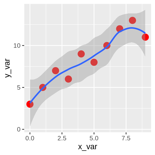
Next, we use R to make a plot using ggplot2 for the above dataframe.

In the first line, we call R using %%R magic where

• -i is our dataframe input

• -w and -h define figure size

• -units in -r define size units in resolution, e.g. 200 dpi in this example. Unit can be changed to px, cm, etc.

Then, we’ll create the plot using the packageggplot2.

3.2.2. Use a native R kernel¶

For a full R notebook experience, install the IRkernel:

Install the IRkernel) package

IRkernel can be installed from CRAN. Run this in a cell with R magic:

Register the kernel with Jupyter

After installation, make the R kernel available to Jupyter:

%%R
IRkernel::installspec()        # Install kernel for the current user

This registers a new kernel with the name ir and display name R.

To install system-wide, set user to FALSE in the installspec command:

Create an R notebook

After installation, create a new notebook and select the R kernel from the kernel dropdown menu. You can now write R code directly without %%R magic.

Which approach should you use?¶

• Use R Magic if you want to use both Python and R in the same notebook without switching kernels

• Use R Kernel if you’re doing extensive R analysis and want a native R notebook experience

3.3. Magics on Python¶

%%writefile Magic

Start Python coding with %%writefile filename.py.

To create a hello.py file (including the function hello), type:

This will save the script to hello.py into your working directory.

Now, to run the code you’ve just saved, use the following in a new cell:

This will execute the hello.py file and call the hello function with “World” as the argument.

You can also load the contents of hello.py directly into a notebook cell using the %load magic command. When you run the cell with %load hello.py, the code from hello.py will be inserted into the cell, allowing you to edit or run it interactively. Note that %load will automatically comment itself out once run, replacing the command with the loaded code.

%%file Magic

%%file magic works similarly to %%writefile. Let’s create a greeting.py file. Type and run the following code:

This will save the function to greeting.py in your workspace. You can then run this file again using the %run magic command, which executes the code in the file as if it were a script.

4. Custom Magic Commands¶

In addition to the built-in magic commands, IPython allows you to define your own custom magic commands. This is useful when you have repetitive tasks that you want to encapsulate in a magic command. See the IPython documentation for a full guide on how to create custom magic commands.

Dependencies in Jupyter/Python¶

• Using the package watermark to document system environment and software versions used in this notebook, alongside the Neurodesktop version extracted from the JUPYTER_IMAGE or NEURODESKTOP_VERSION environment variables.