FreeSurfer

Cortical surface reconstruction and subcortical segmentation with `recon-all`¶

Author: Steffen Bollmann, Michèle Masson-Trottier

Original date: 17 Oct 2024

Last updated: 28 Sep 2026

License:

Note: If this notebook uses neuroimaging tools from Neurocontainers, those tools retain their original licenses. Please see Neurodesk citation guidelines for details.

Citation and Resources¶

Tools included in this workflow¶

FreeSurfer:

Fischl B. (2012). FreeSurfer. NeuroImage, 62(2), 774–781. Fischl (2012)
Dale, A. M., Fischl, B., & Sereno, M. I. (1999). Cortical surface-based analysis. I. Segmentation and surface reconstruction. NeuroImage, 9(2), 179–194. Dale et al. (1999)
Fischl, B., Salat, D. H., Busa, E., et al. (2002). Whole brain segmentation: automated labeling of neuroanatomical structures in the human brain. Neuron, 33(3), 341–355. Fischl et al. (2002)

Dataset¶

MP2RAGE T1-weighted average 7T model (human brain model)

Bollmann, Steffen, Andrew Janke, Lars Marstaller, David Reutens, Kieran O’Brien, and Markus Barth. “MP2RAGE T1-weighted average 7T model” January 1, 2017. doi:10.14264/uql.2017.266

Educational resources¶

FreeSurfer recon-all reference table — every processing stage, flag and output file
FreeSurfer tutorials — the official course material
FreeSurfer output file format reference

Introduction¶

FreeSurfer’s recon-all takes a T1-weighted MRI and produces a brain segmentation, cortical surfaces and regional measurements. Here we work through one example, from loading the software to inspecting the results.

This notebook is for researchers and students who know basic Python or shell commands but are new to FreeSurfer. By the end, you should be able to run a reconstruction, find its outputs and recognise problems that need closer inspection.

Statement of need¶

FreeSurfer produces many images, surfaces and measurements, which can be difficult to interpret when first learning the workflow. This notebook connects each processing stage to its outputs and introduces visual checks before reading regional volumes and cortical thickness. It provides a guided starting point for understanding a reconstruction and recognising when further quality control is needed.

What happens inside recon-all?¶

Stage	Main task	Example outputs
`-autorecon1`	Import, resample, correct intensities and skull-strip	`orig.mgz`, `brainmask.mgz`
`-autorecon2`	Segment tissue and construct cortical surfaces	`aseg.mgz`, `lh.white`
`-autorecon3`	Complete surface registration, parcellation and statistics	`lh.aparc.annot`, `lh.aparc.stats`

We use -all to request the complete workflow. FreeSurfer 8 includes deep-learning tools such as SynthStrip and SynthSeg within this workflow.

Requirements¶

Requirement	Details
Neurodesk module	`freesurfer/8.2.0`
Licence	The selected container bundles a licence; verify it below
Python packages	`ipyniivue`, `nibabel`, `numpy`, `pandas`, `matplotlib`, `watermark` from the Neurodesktop base image
Data/storage	Example download: approximately 1.5 GB; allow several GB for reconstruction and QC
Compute	Four CPU threads by default; select CPU and RAM allocations using the note at the start

On a cluster, execute the notebook in a suitably sized allocation and keep THREADS within the allocated CPU count.

Table of contents¶

1. Set up FreeSurfer
2. Download and inspect the input
3. Run recon-all
4. Check the outputs
5. Inspect the images and surfaces
6. Read the measurements

1. Set up FreeSurfer¶

Neurodesk provides FreeSurfer as a module, so no separate installation is needed. We specify the version to keep the example consistent. Use the same version for all subjects in a study.

import module

await module.load('freesurfer/8.2.0')
await module.list()

['freesurfer/8.2.0']

The next cell prints the version reported by FreeSurfer itself. subprocess.run runs a command from Python; check=True stops the notebook if the command fails. We will use it again for the reconstruction.

import subprocess

subprocess.run(["recon-all", "-version"], check=True)

freesurfer-linux-ubuntu22_x86_64-8.2.0-20260314-d932c45

CompletedProcess(args=['recon-all', '-version'], returncode=0)

Import the Python libraries¶

We use NiBabel to read images, pandas to read tables, and matplotlib and NiiVue to display results. These packages are included in Neurodesktop.

import os
from pathlib import Path

import matplotlib.pyplot as plt
import nibabel as nib
import numpy as np
import pandas as pd
from ipyniivue import Mesh, NiiVue

Choose the input and output paths¶

SUBJECTS_DIR contains one folder per subject; SUBJECT_ID names this example’s folder. Use a new subject ID when changing the input or processing version.

For your own 3D T1-weighted image, change INPUT_SCAN and set USE_EXAMPLE = False. For a first run, leave RUN_RECON = True. After completing the reconstruction, set it to False if you want to run the notebook again to inspect the saved results.

USE_EXAMPLE = True
RUN_RECON = True
INPUT_SCAN = Path("mp2rage.nii").resolve()
SUBJECTS_DIR = Path("freesurfer-output").resolve()
SUBJECT_ID = "subjectname"
THREADS = int(os.environ.get("SLURM_CPUS_PER_TASK", "4"))

SUBJECT_DIR = SUBJECTS_DIR / SUBJECT_ID
os.environ["SUBJECTS_DIR"] = str(SUBJECTS_DIR)
print("Results will be written to:", SUBJECT_DIR)

Results will be written to: /home/jovyan/workspace/books/examples/structural_imaging/freesurfer-output/subjectname

Check the licence¶

The selected Neurodesk container includes a FreeSurfer licence. Check it before starting a long run. We print only the licence-file message, not the key.

If you need your own registration key, save it to a file and set os.environ["APPTAINERENV_FS_LICENSE"] to its absolute path before this cell. The prefix passes the setting into the container.

licence = subprocess.run(["testchklc"], capture_output=True, text=True)
for line in (licence.stdout + licence.stderr).splitlines():
    if "license file" in line.lower():
        print(line)
if licence.returncode != 0:
    raise RuntimeError("FreeSurfer licence check failed; configure a licence before continuing")

Trying license file /opt/freesurfer-8.2.0/license.txt
[DEBUG] chklc() 4 line license file /opt/freesurfer-8.2.0/license.txt
4 line license file

2. Download and inspect the input¶

We use the openly available MP2RAGE T1-weighted 7 T average model, cited above. It is a group-average brain, useful for learning the workflow but smoother than an individual scan. Its measurements are not participant-level results.

The download is about 1.5 GB. We first save it with a .part.nii name, then check it before using it as the input. An existing input is checked again without downloading it.

from urllib.request import urlretrieve

DOWNLOAD_URL = "https://imaging.org.au/uploads/Human7T/mp2rageModel_L13_work03-plus-hippocampus-7T-sym-norm-mincanon_v0.8.nii"
scan_to_check = INPUT_SCAN

if USE_EXAMPLE and not INPUT_SCAN.exists():
    INPUT_SCAN.parent.mkdir(parents=True, exist_ok=True)
    scan_to_check = INPUT_SCAN.with_name("mp2rage.part.nii")
    urlretrieve(DOWNLOAD_URL, scan_to_check)
print("Input to inspect:", scan_to_check)

Input to inspect: /home/jovyan/workspace/books/examples/structural_imaging/mp2rage.nii

Read the image header and view the input¶

The header tells us the matrix size and voxel dimensions without loading the entire image into memory. For this example, expect a 640 × 750 × 800 matrix with 0.3 mm voxels. Your own T1 scan can have different dimensions.

img = nib.load(scan_to_check)

print("Matrix:", img.shape)
print("Voxel size:", img.header.get_zooms(), "mm")
print("Data type:", img.get_data_dtype())
print(f"File size: {scan_to_check.stat().st_size / 1e9:.2f} GB")

Matrix: (640, 750, 800)
Voxel size: (np.float32(0.3), np.float32(0.3), np.float32(0.3)) mm
Data type: float32
File size: 1.54 GB

The checks below catch an unexpected image or truncated download before reconstruction. The last-voxel read also checks that the file extends beyond its header. The example-specific dimensions are checked only when USE_EXAMPLE is enabled.

if len(img.shape) != 3:
    raise ValueError("Use a single 3D T1-weighted image")
if not np.isfinite(float(img.dataobj[-1, -1, -1])):
    raise ValueError("The final voxel is not finite")
if USE_EXAMPLE:
    if img.shape != (640, 750, 800) or not np.allclose(img.header.get_zooms(), 0.3):
        raise ValueError("The downloaded example has unexpected dimensions")

if scan_to_check != INPUT_SCAN:
    scan_to_check.rename(INPUT_SCAN)
print("Input check passed")

Input check passed

View a middle slice along each image axis before starting reconstruction. Look for the expected brain coverage, visible tissue contrast and obvious artefacts. These three slices are an initial check, not a complete quality assessment.

The preview reads only the selected slices into memory and preserves their voxel proportions. It uses the image’s native orientation; the axis labels show anatomical directions from the header (L/R: left/right, P/A: posterior/anterior, I/S: inferior/superior). For oblique acquisitions, these are approximate directions.

# Reopen the final path in case the download was renamed after validation.
input_img = nib.load(INPUT_SCAN)
voxel_sizes = input_img.header.get_zooms()
directions = nib.aff2axcodes(input_img.affine)
opposite = {"L": "R", "R": "L", "P": "A", "A": "P", "I": "S", "S": "I"}

fig, axes = plt.subplots(1, 3, figsize=(12, 4), constrained_layout=True)
for axis, ax in enumerate(axes):
    index = input_img.shape[axis] // 2
    selection = [slice(None)] * 3
    selection[axis] = index
    image_slice = np.asarray(input_img.dataobj[tuple(selection)])
    horizontal, vertical = [dimension for dimension in range(3) if dimension != axis]
    ax.imshow(
        image_slice.T, origin="lower", cmap="gray",
        aspect=voxel_sizes[vertical] / voxel_sizes[horizontal],
    )
    ax.set_title(f"Axis {axis}: slice {index}")
    ax.set_xlabel(f"{opposite[directions[horizontal]]} → {directions[horizontal]}")
    ax.set_ylabel(f"{opposite[directions[vertical]]} → {directions[vertical]}")
    ax.set_xticks([])
    ax.set_yticks([])
fig.suptitle("Input image — middle slices")
plt.show()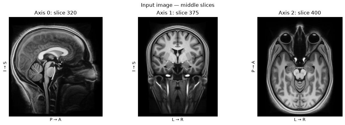

The standard recon-all workflow resamples this high-resolution image to approximately 1 mm voxels. This reduces the detail but matches the standard processing stream. We will view that smaller, conformed image after reconstruction.

3. Run recon-all¶

Before running, create the output directory and check that we will not overwrite a subject. For a fresh reconstruction, use an unused SUBJECT_ID. To inspect a completed subject, use its original paths and set RUN_RECON = False above.

FreeSurfer writes an IsRunning* file while processing. If one is present, first check whether the process is still active. Remove a stale flag only after confirming that no reconstruction is running.

SUBJECTS_DIR.mkdir(parents=True, exist_ok=True)

if list((SUBJECT_DIR / "scripts").glob("IsRunning*")):
    raise RuntimeError("An IsRunning flag exists; check whether FreeSurfer is still running")
if RUN_RECON and SUBJECT_DIR.exists():
    raise FileExistsError("Use a new SUBJECT_ID, or follow the resume instructions below")
if not RUN_RECON and not SUBJECT_DIR.is_dir():
    raise FileNotFoundError("No saved subject exists; set RUN_RECON = True for a first run")

Some FreeSurfer 8 builds require FS_ALLOW_DEEP to enable machine-learning routines. The prefixed variables pass this setting into Neurodesk’s container; it is unrelated to directory depth.

os.environ["FS_ALLOW_DEEP"] = "1"
os.environ["APPTAINERENV_FS_ALLOW_DEEP"] = "1"
os.environ["SINGULARITYENV_FS_ALLOW_DEEP"] = "1"

Start the reconstruction¶

The command below specifies:

-subject: the output subject name;
-i: the input T1 image, imported on the first run;
-all: the complete reconstruction;
-sd: the subjects directory;
-threads: the number of CPU threads.

Expect this cell to take hours. Its output is scrollable, and FreeSurfer also writes scripts/recon-all.log inside the subject directory.

if RUN_RECON:
    subprocess.run([
        "recon-all", "-subject", SUBJECT_ID,
        "-i", str(INPUT_SCAN), "-all",
        "-sd", str(SUBJECTS_DIR), "-threads", str(THREADS),
    ], check=True)
else:
    print("Inspecting saved results; reconstruction was not run")

If the run was interrupted

Inspect scripts/recon-all.log and resolve the reported error first. If import completed (mri/orig/001.mgz exists) and no process is active, resume without -i. In a new notebook code cell, run:

subprocess.run([
    "recon-all", "-subject", SUBJECT_ID, "-all",
    "-sd", str(SUBJECTS_DIR), "-threads", str(THREADS),
], check=True)

Use the same input, subject ID, version and environment. Then continue with Section 4. For later Run All inspections, set RUN_RECON = False. If the initial import failed, preserve the incomplete folder and start with a new subject ID. FreeSurfer documents rerun issues in version 8.0.0, so inspect resumed results carefully.

4. Check the outputs¶

A recon-all.done file alone is not proof of a complete reconstruction: it can describe a subset of stages or an unsuccessful run. Check the completion record and absence of an error file first.

scripts_dir = SUBJECT_DIR / "scripts"
done_file = scripts_dir / "recon-all.done"

if (scripts_dir / "recon-all.error").exists():
    raise RuntimeError("FreeSurfer recorded an error; inspect scripts/recon-all.log")
if not done_file.is_file() or "END_TIME" not in done_file.read_text():
    raise RuntimeError("No successful completion record was found")
print(done_file.read_text())

------------------------------
SUBJECT subjectname
START_TIME Mon Sep 28 07:14:53 AM UTC 2026
END_TIME Mon Sep 28 08:48:03 AM UTC 2026
RUNTIME_HOURS 1.553
USER jovyan
HOST fdd337dada5e
PROCESSOR x86_64
OS Linux
UNAME Linux fdd337dada5e 6.8.0-111-generic #111-Ubuntu SMP PREEMPT_DYNAMIC Sat Apr 11 23:16:02 UTC 2026 x86_64 x86_64 x86_64 GNU/Linux
VERSION 8.2.0 (freesurfer-linux-ubuntu22_x86_64-8.2.0-20260314-d932c45)
CMDPATH /opt/freesurfer-8.2.0/bin/recon-all
CMDARGS -subject subjectname -i /home/jovyan/workspace/books/examples/structural_imaging/mp2rage.nii -all -sd /home/jovyan/workspace/books/examples/structural_imaging/freesurfer-output -threads 4

Now check the files used in the rest of the notebook. Missing files usually mean that processing stopped early or only part of the workflow ran. These checks establish that the outputs are present; visual inspection is still needed to assess their anatomy.

expected_files = [
    "mri/orig.mgz", "mri/brainmask.mgz", "mri/aseg.mgz",
    "surf/lh.white", "surf/rh.white", "surf/lh.pial", "surf/rh.pial",
    "stats/aseg.stats", "stats/lh.aparc.stats", "stats/rh.aparc.stats",
]
for name in expected_files:
    path = SUBJECT_DIR / name
    if not path.is_file() or path.stat().st_size == 0:
        raise FileNotFoundError(f"Missing or empty output: {path}")
print("All files needed for this notebook are present")

All files needed for this notebook are present

The subject folder follows FreeSurfer’s standard layout:

Folder	What to look for
`mri/`	`orig.mgz`: conformed input; `brainmask.mgz`: extracted brain; `aseg.mgz`: labelled structures
`surf/`	`lh.white` and `rh.white`: grey/white boundaries; `lh.pial` and `rh.pial`: outer cortical boundaries
`label/`	Cortical parcellations such as `lh.aparc.annot`
`stats/`	Subcortical volumes and cortical thickness, area and volume tables
`scripts/`	Processing logs, software build and completion/error records

lh and rh mean left and right hemisphere. The distance between the white and pial surfaces is used to estimate cortical thickness.

5. Inspect the images and surfaces¶

Load the anatomy and segmentation¶

orig.mgz is the conformed anatomical image. In aseg.mgz, each integer identifies a structure. We check that their shapes and spatial transforms agree before displaying them together.

anatomy = nib.load(SUBJECT_DIR / "mri/orig.mgz")
segmentation = nib.load(SUBJECT_DIR / "mri/aseg.mgz")

if anatomy.shape != segmentation.shape or not np.allclose(anatomy.affine, segmentation.affine):
    raise ValueError("The anatomy and segmentation do not share a voxel grid")
print("Conformed image:", anatomy.shape, anatomy.header.get_zooms(), "mm")

Conformed image: (np.int32(256), np.int32(256), np.int32(256)) (np.float32(1.0), np.float32(1.0), np.float32(1.0)) mm

Explore the labelled structures¶

Move through the slices in NiiVue. Check whether the ventricles follow their anatomical boundaries, whether labels extend outside the brain, and whether unexpected asymmetries need closer inspection. Symmetry alone is not a measure of quality.

nv_aseg = NiiVue(height=500, is_colorbar=False)
nv_aseg.load_volumes([
    {"path": str(SUBJECT_DIR / "mri/orig.mgz"), "colormap": "gray"},
    {"path": str(SUBJECT_DIR / "mri/aseg.mgz"), "colormap": "freesurfer",
     "cal_min": 0, "cal_max": 255, "opacity": 0.5},
])
nv_aseg

[HF-patcher] orig: path → url
[HF-patcher] aseg: path → url

A static QC image¶

This slice remains visible when the saved notebook is published without a running kernel. We orient the volumes to RAS so the axial panel has the participant’s left on the left. Set slice_number to inspect another level. The plot uses a display colour map; use the NiiVue view above for FreeSurfer’s label colours.

brain = nib.as_closest_canonical(anatomy).get_fdata()
labels = nib.as_closest_canonical(segmentation).get_fdata()
slice_number = brain.shape[2] // 2

fig, ax = plt.subplots(figsize=(6, 6))
ax.imshow(brain[:, :, slice_number].T, origin="lower", cmap="gray")
label_slice = np.ma.masked_equal(labels[:, :, slice_number].T, 0)
ax.imshow(label_slice, origin="lower", cmap="tab20", alpha=0.4, interpolation="nearest")
ax.set_title(f"Axial slice {slice_number} — participant's left is on the left")
ax.axis("off")
plt.show()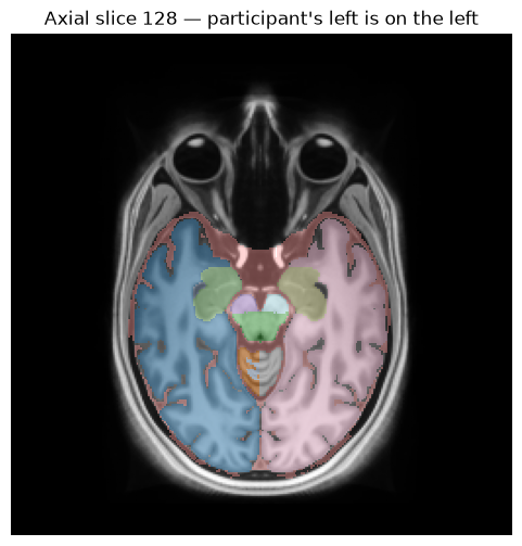

Inspect the cortical surfaces¶

Rotate the pial meshes to look for holes, missing regions or large bulges. This helps find gross defects, but a detached mesh cannot show whether the boundary follows the underlying tissue correctly.

surf_dir = SUBJECT_DIR / "surf"
nv_surf = NiiVue(height=500, is_colorbar=False)
nv_surf.add_mesh(Mesh(path=str(surf_dir / "lh.pial"), rgba255=[255, 90, 90, 255]))
nv_surf.add_mesh(Mesh(path=str(surf_dir / "rh.pial"), rgba255=[90, 90, 255, 255]))
nv_surf

[HF-patcher] lh.pial: path → url
[HF-patcher] rh.pial: path → url

Together, the segmentation slices and pial meshes provide an initial visual check of the reconstruction. The mesh view shows overall surface shape, but does not establish that the white and pial boundaries follow the underlying anatomy. That requires inspecting both boundaries overlaid on the anatomical image across multiple slices.

Next, we read the regional volumes and cortical thickness estimates. Treat these measurements as outputs to inspect alongside the images, rather than evidence by themselves that the reconstruction is accurate.

6. Read the measurements¶

Subcortical volumes¶

aseg.stats is a text file with comments followed by one row per structure. pd.read_csv reads whitespace-separated columns; comment="#" skips the explanatory header. The column names below follow FreeSurfer’s table format.

aseg_columns = [
    "Index", "SegId", "NVoxels", "Volume_mm3", "StructName",
    "normMean", "normStdDev", "normMin", "normMax", "normRange",
]
aseg_table = pd.read_csv(
    SUBJECT_DIR / "stats/aseg.stats", sep=r"\s+", comment="#", names=aseg_columns,
)
aseg_table[["StructName", "Volume_mm3"]].head()

Sort by volume to inspect the largest labelled structures. These values can prompt further image review, but they do not tell you whether the boundaries are anatomically accurate.

aseg_table[["StructName", "Volume_mm3", "NVoxels"]].sort_values(
    "Volume_mm3", ascending=False,
).head(12)

Whole-brain measures are stored separately in the header. The lines below show brain segmentation volume and estimated intracranial volume (eTIV). Head size matters when comparing regional volumes between participants; choosing the appropriate adjustment belongs to the study’s analysis plan.

for line in (SUBJECT_DIR / "stats/aseg.stats").read_text().splitlines():
    if line.startswith("# Measure") and (", eTIV," in line or ", BrainSegVol," in line):
        print(line.removeprefix("# Measure "))

BrainSeg, BrainSegVol, Brain Segmentation Volume, 1455275.000000, mm^3
EstimatedTotalIntraCranialVol, eTIV, Estimated Total Intracranial Volume, 1613288.794666, mm^3

Cortical thickness¶

Each hemisphere has its own aparc.stats file. Read the left hemisphere below; change hemisphere to "rh" to explore the right. ThickAvg is each region’s average thickness in millimetres, not a whole-brain mean.

hemisphere = "lh"
cortical_columns = [
    "StructName", "NumVert", "SurfArea", "GrayVol", "ThickAvg",
    "ThickStd", "MeanCurv", "GausCurv", "FoldInd", "CurvInd",
]
cortical_table = pd.read_csv(
    SUBJECT_DIR / "stats" / f"{hemisphere}.aparc.stats",
    sep=r"\s+", comment="#", names=cortical_columns,
)
cortical_table[["StructName", "ThickAvg", "SurfArea", "GrayVol"]].head(10)

Thickness varies with region, age, acquisition and processing. Unexpected values are a reason to revisit the surface placement, not a universal pass/fail test. Remember that this example uses a group-average brain.

Where to go next¶

Use asegstats2table and aparcstats2table to collect measurements across a cohort.
Follow the FreeSurfer tutorials for manual corrections and detailed QC.
For clinical acquisitions, see recon-all-clinical.
For projecting fMRI data onto surfaces, see mri_vol2surf.

Dependencies in Jupyter/Python¶

The watermark records the Python environment used for this notebook. Keep it with the FreeSurfer version printed at the start when sharing your results.

%load_ext watermark
%watermark
%watermark --iversions

neurodesktop_version = (
    os.environ.get("JUPYTER_IMAGE", "").split(":")[-1]
    or os.environ.get("NEURODESKTOP_VERSION", "unknown")
)
print("Neurodesktop version:", neurodesktop_version)

Last updated: 2026-09-28T08:48:31.489124+00:00

Python implementation: CPython
Python version       : 3.13.14
IPython version      : 9.12.0

Compiler    : GCC 14.3.0
OS          : Linux
Release     : 6.8.0-111-generic
Machine     : x86_64
Processor   : x86_64
CPU cores   : 16
Architecture: 64bit

ipyniivue : 2.4.4
json      : 2.0.9
matplotlib: 3.11.0
nibabel   : 5.4.2
numpy     : 2.5.1
pandas    : 2.3.3

Neurodesktop version: 2026-07-11

References¶

Fischl, B. (2012). FreeSurfer. NeuroImage, 62(2), 774–781. 10.1016/j.neuroimage.2012.01.021
Dale, A. M., Fischl, B., & Sereno, M. I. (1999). Cortical Surface-Based Analysis. NeuroImage, 9(2), 179–194. 10.1006/nimg.1998.0395
Fischl, B., Salat, D. H., Busa, E., Albert, M., Dieterich, M., Haselgrove, C., van der Kouwe, A., Killiany, R., Kennedy, D., Klaveness, S., Montillo, A., Makris, N., Rosen, B., & Dale, A. M. (2002). Whole Brain Segmentation. Neuron, 33(3), 341–355. 10.1016/s0896-6273(02)00569-x

Cortical surface reconstruction and subcortical segmentation with recon-all¶

Citation and Resources¶

Tools included in this workflow¶

Dataset¶

Educational resources¶

Introduction¶

Statement of need¶

What happens inside recon-all?¶

Requirements¶

Table of contents¶

1. Set up FreeSurfer¶

Import the Python libraries¶

Choose the input and output paths¶

Check the licence¶

2. Download and inspect the input¶

Read the image header and view the input¶

3. Run recon-all¶

Start the reconstruction¶

4. Check the outputs¶

5. Inspect the images and surfaces¶

Load the anatomy and segmentation¶

Explore the labelled structures¶

A static QC image¶

Inspect the cortical surfaces¶

6. Read the measurements¶

Subcortical volumes¶

Cortical thickness¶

Where to go next¶

Dependencies in Jupyter/Python¶

Cortical surface reconstruction and subcortical segmentation with `recon-all`¶