Run this notebook
Date: 25 Aug 2025
License:
Note: If this notebook uses neuroimaging tools from Neurocontainers, those tools retain their original licenses. Please see Neurodesk citation guidelines for details.
Citation and Resources:
Tools included in this workflow
QSMxT: Stewart AW, Robinson SD, O’Brien K, et al. QSMxT: Robust masking and artifact reduction for quantitative susceptibility mapping. Magnetic Resonance in Medicine. 2022;87(3):1289-1300. Stewart et al. (2021)
QSMxT: Stewart AW, Bollman S, et al. QSMxT/QSMxT. GitHub; 2022. https://github.com/QSMxT/QSM
Dataset
Bollmann, S., & Stewart, A. (2023, August 7). QSM DICOM testdata for QSMxT pipeline. Retrieved from osf.io/ru43c
QSMxT Interactive Notebook
This interactive notebook estimates Quantitative Susceptibility Maps (QSMs) for two gradient-echo (GRE) MRI acquisitions using QSMxT provided by the Neurodesk project.
What is QSM?
QSM is a form of quantitative MRI (qMRI) that estimates the magnetic susceptibility distribution across an imaged object. Magnetic susceptibility is the degree to which a material becomes magnetised by an external magnetic field. Major contributors to susceptibility include iron, calcium, and myelin, with the susceptibility of water typically approximating a zero-reference, though it is slightly diamagnetic. Read more about QSM here.
What is QSMxT?
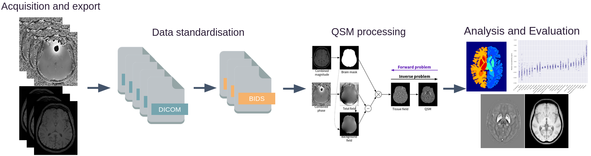
QSMxT is a suite of tools for building and running automated pipelines for QSM that:
is available open-source without any licensing required;
is distributed as a software container making it straightforward to access and install (Neurodesk!)
scales its processing to execute across many acquisitions through jobs parallelisation (using multiple processors or HPCs) provided by Nipype;
automates steps that usually require manual intervention and scripting, including:
DICOM to BIDS conversion;
QSM reconstruction using a range of algorithms;
segmentation using FastSurfer;
group space generation using ANTs;
export of susceptibility statistics by subject and region of interest (ROI) to CSV.
How do I access QSMxT?
There are a few ways you can access QSMxT:
This notebook: You can access QSMxT in this notebook right now!
If you are running this on a Neurodesk Play instance, you can upload your own data into the sidebar via drag-and-drop.
Neurodesktop: QSMxT is in the applications menu of Neurodesktop.
On Neurodesk Play, upload your own data into the desktop via drag-and-drop.
On a local install of Neurodesk, bring any necessary files into the shared
~/neurodesktop-storagedirectory
Local install: QSMxT can also be installed via the Docker container
HPC install: QSMxT can also be installed via the Singularity container for use on HPCs
Download example DICOMs
Here, we download some example DICOMs from our OSF repository for QSMxT, through its HuggingFace mirror.
These data include GRE and T1-weighted acquisitions for one subject (duplicated to act as two subjects).
!curl -fL --retry 5 --retry-all-errors -sS -o dicoms-unsorted.tar https://huggingface.co/datasets/neurodeskorg/qsm-testdata/resolve/c97dfec3f16c6f4b5570e260a323931ed48db9ef/dicoms-unsorted.tar
!tar xf dicoms-unsorted.tar
!rm dicoms-unsorted.tar
!tree dicoms-unsorted | head
!echo -e "...\nThere are `ls dicoms-unsorted | wc -l` unsorted DICOMs in ./dicoms-unsorted/"
dicoms-unsorted
├── MR.1.1.dcm
├── MR.1.10.dcm
├── MR.1.100.dcm
├── MR.1.101.dcm
├── MR.1.102.dcm
├── MR.1.103.dcm
├── MR.1.104.dcm
├── MR.1.105.dcm
├── MR.1.106.dcm
...
There are 1216 unsorted DICOMs in ./dicoms-unsorted/
Load QSMxT
To load QSMxT inside a notebook, we can use the available module system:
import module
await module.load('qsmxt/8.1.1')
!qsmxt --version
[INFO]: QSMxT v8.1.1
Data standardisation
QSMxT requires input data to conform to the Brain Imaging Data Structure (BIDS).
Luckily, QSMxT also provides scripts that can convert unorganised NIfTI or DICOM images to BIDS. If you are using NIfTI images and do not have DICOMs, see nifti-convert.
Convert DICOM to BIDS
The DICOM to BIDS conversion must identify which series should be used for QSM reconstruction (e.g. MEGRE), and which series should be used for segmentation (T1-weighted). Because this information is not stored in the DICOM header in a standardised way, it can only be estimated based on other fields, or the user must identify series themselves.
If QSMxT is run interactively, the user will be prompted to identify the relevant series. However, because we are running QSMxT in a notebook, we disable the interactivity using --auto_yes and allow QSMxT to guess the intended purpose of each acquisition. In this case, it makes the right guess:
!dicom-convert dicoms-unsorted bids --auto_yes/opt/miniconda-4.12.0/lib/python3.8/site-packages/dicompare/io.py:30: UserWarning: The DICOM readers are highly experimental, unstable, and only work for Siemens time-series at the moment
Please use with caution. We would be grateful for your help in improving them
from nibabel.nicom.csareader import get_csa_header
[INFO]: Running QSMxT 8.1.1
[INFO]: Command: /opt/miniconda-4.12.0/bin/dicom-convert dicoms-unsorted bids --auto_yes
[INFO]: Python interpreter: /opt/miniconda-4.12.0/bin/python3.8
Loading DICOM files: 100%|█████████████████| 1216/1216 [00:11<00:00, 101.91it/s]
[INFO]: Loaded DICOM session in 12.10 seconds
/opt/miniconda-4.12.0/lib/python3.8/site-packages/dicompare/acquisition.py:144: PerformanceWarning: DataFrame is highly fragmented. This is usually the result of calling `frame.insert` many times, which has poor performance. Consider joining all columns at once using pd.concat(axis=1) instead. To get a de-fragmented frame, use `newframe = frame.copy()`
session_df["BaseAcquisition"] = "acq-" + session_df[acquisition_fields].apply(
/opt/miniconda-4.12.0/lib/python3.8/site-packages/dicompare/acquisition.py:195: PerformanceWarning: DataFrame is highly fragmented. This is usually the result of calling `frame.insert` many times, which has poor performance. Consider joining all columns at once using pd.concat(axis=1) instead. To get a de-fragmented frame, use `newframe = frame.copy()`
session_df.loc[param_group.index, "AcquisitionSignature"] = signature
/opt/miniconda-4.12.0/lib/python3.8/site-packages/dicompare/acquisition.py:218: PerformanceWarning: DataFrame is highly fragmented. This is usually the result of calling `frame.insert` many times, which has poor performance. Consider joining all columns at once using pd.concat(axis=1) instead. To get a de-fragmented frame, use `newframe = frame.copy()`
session_df["RunNumber"] = 1
/opt/miniconda-4.12.0/lib/python3.8/site-packages/dicompare/acquisition.py:301: PerformanceWarning: DataFrame is highly fragmented. This is usually the result of calling `frame.insert` many times, which has poor performance. Consider joining all columns at once using pd.concat(axis=1) instead. To get a de-fragmented frame, use `newframe = frame.copy()`
session_df["Acquisition"] = session_df["AcquisitionSignature"].fillna("Unknown").astype(str)
[INFO]: Auto-assigning initial labels
[INFO]: Auto-assigned selections:
Acquisition ... Description
0 acq-mp2ragehighres0p5isoslab ...
1 acq-qsmp21mmisote20 ...
2 acq-qsmp21mmisote20 ...
[3 rows x 7 columns]
[INFO]: Merging selections into dataframe...
[INFO]: Processing base group: ('dev_siemens^SB', 1, 20170705, 'acq-mp2ragehighres0p5isoslab', 'mp2rage_highRes_0p5iso_slab_UNI-DEN', 1, '1.2.276.0.7230010.3.1.3.0.4480.1677042698.772469', 'NA')
[INFO]: Found 1 unique Types in this group
[INFO]: Processing Type group: T1w with 288 rows
[INFO]: Found multiple DICOM paths for Type 'T1w', grouping by EchoNumber
[INFO]: Processing Echo group: 1.0 with 288 rows
[INFO]: Converting group with 288 rows
[INFO]: Running command: '"dcm2niix" -o "/home/jovyan/workspace/books/examples/quantitative_imaging/bids/temp_convert" -f "temp_output" -z n -m o "/home/jovyan/workspace/books/examples/quantitative_imaging/bids/temp_convert"'
Chris Rorden's dcm2niiX version v1.0.20240202 (JP2:OpenJPEG) (JP-LS:CharLS) GCC11.4.0 x86-64 (64-bit Linux)
Found 288 DICOM file(s)
Convert 288 DICOM as /home/jovyan/workspace/books/examples/quantitative_imaging/bids/temp_convert/temp_output (378x420x288x1)
Conversion required 0.633146 seconds (0.630892 for core code).
[INFO]: Processing base group: ('dev_siemens^SB', 1, 20170705, 'acq-qsmp21mmisote20', 'QSM_p2_1mmIso_TE20', 1, '1.3.12.2.1107.5.2.43.167001.2017070513471948579426649.0.0.0', 'HC1-7')
[INFO]: Found 1 unique Types in this group
[INFO]: Processing Type group: Mag with 160 rows
[INFO]: Found multiple DICOM paths for Type 'Mag', grouping by EchoNumber
[INFO]: Processing Echo group: 1.0 with 160 rows
[INFO]: Converting group with 160 rows
[INFO]: Running command: '"dcm2niix" -o "/home/jovyan/workspace/books/examples/quantitative_imaging/bids/temp_convert" -f "temp_output" -z n -m o "/home/jovyan/workspace/books/examples/quantitative_imaging/bids/temp_convert"'
Chris Rorden's dcm2niiX version v1.0.20240202 (JP2:OpenJPEG) (JP-LS:CharLS) GCC11.4.0 x86-64 (64-bit Linux)
Found 160 DICOM file(s)
Convert 160 DICOM as /home/jovyan/workspace/books/examples/quantitative_imaging/bids/temp_convert/temp_output (224x224x160x1)
Conversion required 0.136193 seconds (0.133338 for core code).
[INFO]: Processing base group: ('dev_siemens^SB', 1, 20170705, 'acq-qsmp21mmisote20', 'QSM_p2_1mmIso_TE20', 1, '1.3.12.2.1107.5.2.43.167001.2017070513471948580526650.0.0.0', 'HC1-7')
[INFO]: Found 1 unique Types in this group
[INFO]: Processing Type group: Phase with 160 rows
[INFO]: Found multiple DICOM paths for Type 'Phase', grouping by EchoNumber
[INFO]: Processing Echo group: 1.0 with 160 rows
[INFO]: Converting group with 160 rows
[INFO]: Running command: '"dcm2niix" -o "/home/jovyan/workspace/books/examples/quantitative_imaging/bids/temp_convert" -f "temp_output" -z n -m o "/home/jovyan/workspace/books/examples/quantitative_imaging/bids/temp_convert"'
Chris Rorden's dcm2niiX version v1.0.20240202 (JP2:OpenJPEG) (JP-LS:CharLS) GCC11.4.0 x86-64 (64-bit Linux)
Found 160 DICOM file(s)
Convert 160 DICOM as /home/jovyan/workspace/books/examples/quantitative_imaging/bids/temp_convert/temp_output_ph (224x224x160x1)
Conversion required 0.129451 seconds (0.129365 for core code).
[INFO]: Processing base group: ('dev_siemens^SB', 2, 20170705, 'acq-mp2ragehighres0p5isoslab', 'mp2rage_highRes_0p5iso_slab_UNI-DEN', 1, 2, 'NA')
[INFO]: Found 1 unique Types in this group
[INFO]: Processing Type group: T1w with 288 rows
[INFO]: Found multiple DICOM paths for Type 'T1w', grouping by EchoNumber
[INFO]: Processing Echo group: 1.0 with 288 rows
[INFO]: Converting group with 288 rows
[INFO]: Running command: '"dcm2niix" -o "/home/jovyan/workspace/books/examples/quantitative_imaging/bids/temp_convert" -f "temp_output" -z n -m o "/home/jovyan/workspace/books/examples/quantitative_imaging/bids/temp_convert"'
Chris Rorden's dcm2niiX version v1.0.20240202 (JP2:OpenJPEG) (JP-LS:CharLS) GCC11.4.0 x86-64 (64-bit Linux)
Found 288 DICOM file(s)
Convert 288 DICOM as /home/jovyan/workspace/books/examples/quantitative_imaging/bids/temp_convert/temp_output (378x420x288x1)
Conversion required 0.543082 seconds (0.543002 for core code).
[INFO]: Processing base group: ('dev_siemens^SB', 2, 20170705, 'acq-qsmp21mmisote20', 'QSM_p2_1mmIso_TE20', 1, 1, 'HC1-7')
[INFO]: Found 1 unique Types in this group
[INFO]: Processing Type group: Mag with 160 rows
[INFO]: Found multiple DICOM paths for Type 'Mag', grouping by EchoNumber
[INFO]: Processing Echo group: 1.0 with 160 rows
[INFO]: Converting group with 160 rows
[INFO]: Running command: '"dcm2niix" -o "/home/jovyan/workspace/books/examples/quantitative_imaging/bids/temp_convert" -f "temp_output" -z n -m o "/home/jovyan/workspace/books/examples/quantitative_imaging/bids/temp_convert"'
Chris Rorden's dcm2niiX version v1.0.20240202 (JP2:OpenJPEG) (JP-LS:CharLS) GCC11.4.0 x86-64 (64-bit Linux)
Found 160 DICOM file(s)
Convert 160 DICOM as /home/jovyan/workspace/books/examples/quantitative_imaging/bids/temp_convert/temp_output (224x224x160x1)
Conversion required 0.128328 seconds (0.128272 for core code).
[INFO]: Processing base group: ('dev_siemens^SB', 2, 20170705, 'acq-qsmp21mmisote20', 'QSM_p2_1mmIso_TE20', 1, 3, 'HC1-7')
[INFO]: Found 1 unique Types in this group
[INFO]: Processing Type group: Phase with 160 rows
[INFO]: Found multiple DICOM paths for Type 'Phase', grouping by EchoNumber
[INFO]: Processing Echo group: 1.0 with 160 rows
[INFO]: Converting group with 160 rows
[INFO]: Running command: '"dcm2niix" -o "/home/jovyan/workspace/books/examples/quantitative_imaging/bids/temp_convert" -f "temp_output" -z n -m o "/home/jovyan/workspace/books/examples/quantitative_imaging/bids/temp_convert"'
Chris Rorden's dcm2niiX version v1.0.20240202 (JP2:OpenJPEG) (JP-LS:CharLS) GCC11.4.0 x86-64 (64-bit Linux)
Found 160 DICOM file(s)
Convert 160 DICOM as /home/jovyan/workspace/books/examples/quantitative_imaging/bids/temp_convert/temp_output_ph (224x224x160x1)
Conversion required 0.130786 seconds (0.126136 for core code).
[INFO]: Scanning for multi-coil data to merge...
[INFO]: Scanning for multi-coil runs to combine...
[INFO]: Checking for complex or polar data requiring fixing...
Loading NIfTIs: 100%|█████████████████████████| 46/46 [00:00<00:00, 1297.11it/s]
[INFO]: Finished
!tree bidsInspect input data
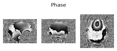
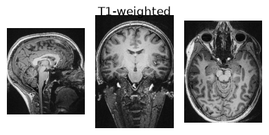
Here we define a function we will use to visualise NIfTI images so we can view some of the input data:
%%capture
!pip install seaborn==0.13.2 numpy==2.3.5 nibabel==5.3.3 pandas==2.3.3 nilearn==0.13.1
from glob import glob
from matplotlib import pyplot as plt
import numpy as np
import nibabel as nib
def show_nii(nii_path, title=None, figsize=(4,5), cmap='gray', **imshow_args):
# load data\n",
data_1 = nib.load(nii_path).get_fdata()
# get middle slices\n",
slc_data1 = np.rot90(data_1[np.shape(data_1)[0]//2,:,:])
slc_data2 = np.rot90(data_1[:,np.shape(data_1)[1]//2,:])
slc_data3 = np.rot90(data_1[:,:,np.shape(data_1)[2]//2])
# show slices\n",
fig, axes = plt.subplots(nrows=1, ncols=3, figsize=figsize)
if title: plt.suptitle(title)
axes[0].imshow(slc_data1, cmap=cmap, **imshow_args)
axes[1].imshow(slc_data2, cmap=cmap, **imshow_args)
axes[2].imshow(slc_data3, cmap=cmap, **imshow_args)
axes[0].axis('off')
axes[1].axis('off')
axes[2].axis('off')
fig.tight_layout()
fig.subplots_adjust(top=1.55)
plt.show()show_nii(glob("bids/sub-*/ses-*/anat/*mag*T2starw*nii*")[0], title="Magnitude", vmax=500)
show_nii(glob("bids/sub-*/ses-*/anat/*phase*T2starw*nii*")[0], title="Phase")
show_nii(glob("bids/sub-*/ses-*/anat/*T1w*nii*")[0], title="T1-weighted")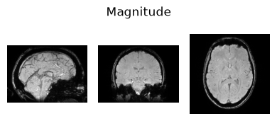
Interactive Display using Niivue
from ipyniivue import NiiVue

nv_T1 = NiiVue()
nv_T1.load_volumes([{"path": glob("bids/sub-*/ses-*/anat/*T1w*nii*")[0]}])
nv_T1
[HF-patcher] sub-2: path → url
Run QSMxT
We are now ready to run QSMxT! We will generate susceptibility maps and segmentations, and export analysis CSVs to file.
The usual way of running QSMxT is to use qsmxt bids_dir. This will launch an interactive command-line interface (CLI) to setup your desired pipelines. However, since we are running this in a notebook, we need to use command-line arguments to by-pass the interface and execute a pipeline.
But first, let’s consider our pipeline settings. For QSM reconstruction, QSMxT provides a range of sensible defaults fit for different purposes. We can list the premade QSM pipelines using --list_premades. For the full pipeline details used for each premade pipeline, see qsm_pipelines.json.
!qsmxt --list_premades=== Premade pipelines ===
default: Default QSMxT settings (GRE; assumes human brain)
gre: Applies suggested settings for 3D-GRE images
epi: Applies suggested settings for 3D-EPI images (assumes human brain)
bet: Applies a traditional BET-masking approach (artefact reduction unavailable; assumes human brain)
fast: Applies a set of fast algorithms
body: Applies suggested settings for non-brain applications
nextqsm: Applies suggested settings for running the NeXtQSM algorithm (assumes human brain)
[INFO]: Finished
For this demonstration, we will go with the fast pipeline. To export segmentations and analysis results, we will use --do_segmentation and --do_analysis. The --auto_yes option avoid the interactive CLI interface that cannot be used in a notebook:
!qsmxt bids \
    --premade fast \
    --do_qsm \
    --do_segmentation \
    --do_analysis \
--auto_yesView results
Let’s have a look at the generated qsm folder:
!tree bids/derivatives/qsmxt-*-* --dirsfirstbids/derivatives/qsmxt-2026-10-07-121200
├── sub-1
│ └── ses-20170705
│ ├── anat
│ │ ├── sub-1_ses-20170705_acq-acqmp2ragehighres0p5isoslab_T1w_space-orig_dseg.nii
│ │ ├── sub-1_ses-20170705_acq-acqmp2ragehighres0p5isoslab_T1w_space-qsm_dseg.nii
│ │ ├── sub-1_ses-20170705_acq-acqqsmp21mmisote20_T2starw_Chimap.json
│ │ ├── sub-1_ses-20170705_acq-acqqsmp21mmisote20_T2starw_Chimap.nii
│ │ ├── sub-1_ses-20170705_acq-acqqsmp21mmisote20_T2starw_space-orig_dseg.nii
│ │ └── sub-1_ses-20170705_acq-acqqsmp21mmisote20_T2starw_space-qsm_dseg.nii
│ └── extra_data
│ ├── sub-1_ses-20170705_acq-acqmp2ragehighres0p5isoslab_T1w_desc-t1w-to-qsm_transform.mat
│ ├── sub-1_ses-20170705_acq-acqqsmp21mmisote20_T2starw_desc-t1w-to-qsm_transform.mat
│ └── sub-1_ses-20170705_acq-acqqsmp21mmisote20_T2starw_qsm-analysis.csv
├── sub-2
│ └── ses-20170705
│ ├── anat
│ │ ├── sub-2_ses-20170705_acq-acqmp2ragehighres0p5isoslab_T1w_space-orig_dseg.nii
│ │ ├── sub-2_ses-20170705_acq-acqmp2ragehighres0p5isoslab_T1w_space-qsm_dseg.nii
│ │ ├── sub-2_ses-20170705_acq-acqqsmp21mmisote20_T2starw_Chimap.json
│ │ ├── sub-2_ses-20170705_acq-acqqsmp21mmisote20_T2starw_Chimap.nii
│ │ ├── sub-2_ses-20170705_acq-acqqsmp21mmisote20_T2starw_space-orig_dseg.nii
│ │ └── sub-2_ses-20170705_acq-acqqsmp21mmisote20_T2starw_space-qsm_dseg.nii
│ └── extra_data
│ ├── sub-2_ses-20170705_acq-acqmp2ragehighres0p5isoslab_T1w_desc-t1w-to-qsm_transform.mat
│ ├── sub-2_ses-20170705_acq-acqqsmp21mmisote20_T2starw_desc-t1w-to-qsm_transform.mat
│ └── sub-2_ses-20170705_acq-acqqsmp21mmisote20_T2starw_qsm-analysis.csv
├── command.txt
├── pypeline.log
├── qsmxt.log
├── references.txt
└── settings.json
bids/derivatives/qsmxt-2026-10-07-123439
├── sub-1
│ └── ses-20170705
│ ├── anat
│ │ ├── sub-1_ses-20170705_acq-acqmp2ragehighres0p5isoslab_T1w_space-orig_dseg.nii
│ │ ├── sub-1_ses-20170705_acq-acqmp2ragehighres0p5isoslab_T1w_space-qsm_dseg.nii
│ │ ├── sub-1_ses-20170705_acq-acqqsmp21mmisote20_T2starw_Chimap.json
│ │ ├── sub-1_ses-20170705_acq-acqqsmp21mmisote20_T2starw_Chimap.nii
│ │ ├── sub-1_ses-20170705_acq-acqqsmp21mmisote20_T2starw_space-orig_dseg.nii
│ │ └── sub-1_ses-20170705_acq-acqqsmp21mmisote20_T2starw_space-qsm_dseg.nii
│ └── extra_data
│ ├── sub-1_ses-20170705_acq-acqqsmp21mmisote20_T2starw_qsm-analysis
│ │ ├── sub-1_ses-20170705_acq-acqqsmp21mmisote20_T2starw_desc-qsmxt-2026-10-07-121200_Chimap_sub-1_ses-20170705_acq-acqqsmp21mmisote20_T2starw_space-qsm_desc-qsmxt-2026-10-07-121200_dseg_analysis.csv
│ │ ├── sub-1_ses-20170705_acq-acqqsmp21mmisote20_T2starw_desc-qsmxt-2026-10-07-121200_Chimap_sub-1_ses-20170705_space-qsm_desc-qsmxt-2026-10-07-123439_dseg_analysis.csv
│ │ ├── sub-1_ses-20170705_desc-qsmxt-2026-10-07-123439_Chimap_sub-1_ses-20170705_acq-acqqsmp21mmisote20_T2starw_space-qsm_desc-qsmxt-2026-10-07-121200_dseg_analysis.csv
│ │ └── sub-1_ses-20170705_desc-qsmxt-2026-10-07-123439_Chimap_sub-1_ses-20170705_space-qsm_desc-qsmxt-2026-10-07-123439_dseg_analysis.csv
│ ├── sub-1_ses-20170705_acq-acqmp2ragehighres0p5isoslab_T1w_desc-t1w-to-qsm_transform.mat
│ └── sub-1_ses-20170705_acq-acqqsmp21mmisote20_T2starw_desc-t1w-to-qsm_transform.mat
├── sub-2
│ └── ses-20170705
│ ├── anat
│ │ ├── sub-2_ses-20170705_acq-acqmp2ragehighres0p5isoslab_T1w_space-orig_dseg.nii
│ │ ├── sub-2_ses-20170705_acq-acqmp2ragehighres0p5isoslab_T1w_space-qsm_dseg.nii
│ │ ├── sub-2_ses-20170705_acq-acqqsmp21mmisote20_T2starw_Chimap.json
│ │ ├── sub-2_ses-20170705_acq-acqqsmp21mmisote20_T2starw_Chimap.nii
│ │ ├── sub-2_ses-20170705_acq-acqqsmp21mmisote20_T2starw_space-orig_dseg.nii
│ │ └── sub-2_ses-20170705_acq-acqqsmp21mmisote20_T2starw_space-qsm_dseg.nii
│ └── extra_data
│ ├── sub-2_ses-20170705_acq-acqqsmp21mmisote20_T2starw_qsm-analysis
│ │ ├── sub-2_ses-20170705_acq-acqqsmp21mmisote20_T2starw_desc-qsmxt-2026-10-07-121200_Chimap_sub-2_ses-20170705_acq-acqqsmp21mmisote20_T2starw_space-qsm_desc-qsmxt-2026-10-07-121200_dseg_analysis.csv
│ │ ├── sub-2_ses-20170705_acq-acqqsmp21mmisote20_T2starw_desc-qsmxt-2026-10-07-121200_Chimap_sub-2_ses-20170705_space-qsm_desc-qsmxt-2026-10-07-123439_dseg_analysis.csv
│ │ ├── sub-2_ses-20170705_desc-qsmxt-2026-10-07-123439_Chimap_sub-2_ses-20170705_acq-acqqsmp21mmisote20_T2starw_space-qsm_desc-qsmxt-2026-10-07-121200_dseg_analysis.csv
│ │ └── sub-2_ses-20170705_desc-qsmxt-2026-10-07-123439_Chimap_sub-2_ses-20170705_space-qsm_desc-qsmxt-2026-10-07-123439_dseg_analysis.csv
│ ├── sub-2_ses-20170705_acq-acqmp2ragehighres0p5isoslab_T1w_desc-t1w-to-qsm_transform.mat
│ └── sub-2_ses-20170705_acq-acqqsmp21mmisote20_T2starw_desc-t1w-to-qsm_transform.mat
├── command.txt
├── pypeline.log
├── qsmxt.log
├── references.txt
└── settings.json
20 directories, 52 files
The references.txt file contains a list of all the algorithms used and relevant citations:
!cat bids/derivatives/qsmxt-*-*/references.txt== References ==
- QSMxT: Stewart AW, Robinson SD, O'Brien K, et al. QSMxT: Robust masking and artifact reduction for quantitative susceptibility mapping. Magnetic Resonance in Medicine. 2022;87(3):1289-1300. doi:10.1002/mrm.29048
- QSMxT: Stewart AW, Bollman S, et al. QSMxT/QSMxT. GitHub; 2022. https://github.com/QSMxT/QSMxT
- Python package - Nipype: Gorgolewski K, Burns C, Madison C, et al. Nipype: A Flexible, Lightweight and Extensible Neuroimaging Data Processing Framework in Python. Frontiers in Neuroinformatics. 2011;5. Accessed April 20, 2022. doi:10.3389/fninf.2011.00013
- Brain extraction: Smith SM. Fast robust automated brain extraction. Human Brain Mapping. 2002;17(3):143-155. doi:10.1002/hbm.10062
- Brain extraction: Liangfu Chen. liangfu/bet2 - Standalone Brain Extraction Tool. GitHub; 2015. https://github.com/liangfu/bet2
- Unwrapping algorithm - ROMEO: Dymerska B, Eckstein K, Bachrata B, et al. Phase unwrapping with a rapid opensource minimum spanning tree algorithm (ROMEO). Magnetic Resonance in Medicine. 2021;85(4):2294-2308. doi:10.1002/mrm.28563
- Background field removal - V-SHARP: Wu B, Li W, Guidon A et al. Whole brain susceptibility mapping using compressed sensing. Magnetic resonance in medicine. 2012 Jan;67(1):137-47. doi:10.1002/mrm.23000
- QSM algorithm - RTS: Kames C, Wiggermann V, Rauscher A. Rapid two-step dipole inversion for susceptibility mapping with sparsity priors. Neuroimage. 2018 Feb 15;167:276-83. doi:10.1016/j.neuroimage.2017.11.018
- Julia package - QSM.jl: kamesy. GitHub; 2022. https://github.com/kamesy/QSM.jl
- Julia package - MriResearchTools: Eckstein K. korbinian90/MriResearchTools.jl. GitHub; 2022. https://github.com/korbinian90/MriResearchTools.jl
- Python package - nibabel: Brett M, Markiewicz CJ, Hanke M, et al. nipy/nibabel. GitHub; 2019. https://github.com/nipy/nibabel
- Python package - scipy: Virtanen P, Gommers R, Oliphant TE, et al. SciPy 1.0: fundamental algorithms for scientific computing in Python. Nat Methods. 2020;17(3):261-272. doi:10.1038/s41592-019-0686-2
- Python package - numpy: Harris CR, Millman KJ, van der Walt SJ, et al. Array programming with NumPy. Nature. 2020;585(7825):357-362. doi:10.1038/s41586-020-2649-2
- FastSurfer: Henschel L, Conjeti S, Estrada S, Diers K, Fischl B, Reuter M. FastSurfer - A fast and accurate deep learning based neuroimaging pipeline. NeuroImage. 2020;219:117012. doi:10.1016/j.neuroimage.2020.117012
- ANTs: Avants BB, Tustison NJ, Johnson HJ. Advanced Normalization Tools. GitHub; 2022. https://github.com/ANTsX/ANTs
== References ==
- QSMxT: Stewart AW, Robinson SD, O'Brien K, et al. QSMxT: Robust masking and artifact reduction for quantitative susceptibility mapping. Magnetic Resonance in Medicine. 2022;87(3):1289-1300. doi:10.1002/mrm.29048
- QSMxT: Stewart AW, Bollman S, et al. QSMxT/QSMxT. GitHub; 2022. https://github.com/QSMxT/QSMxT
- Python package - Nipype: Gorgolewski K, Burns C, Madison C, et al. Nipype: A Flexible, Lightweight and Extensible Neuroimaging Data Processing Framework in Python. Frontiers in Neuroinformatics. 2011;5. Accessed April 20, 2022. doi:10.3389/fninf.2011.00013
- Brain extraction: Smith SM. Fast robust automated brain extraction. Human Brain Mapping. 2002;17(3):143-155. doi:10.1002/hbm.10062
- Brain extraction: Liangfu Chen. liangfu/bet2 - Standalone Brain Extraction Tool. GitHub; 2015. https://github.com/liangfu/bet2
- Unwrapping algorithm - ROMEO: Dymerska B, Eckstein K, Bachrata B, et al. Phase unwrapping with a rapid opensource minimum spanning tree algorithm (ROMEO). Magnetic Resonance in Medicine. 2021;85(4):2294-2308. doi:10.1002/mrm.28563
- Background field removal - V-SHARP: Wu B, Li W, Guidon A et al. Whole brain susceptibility mapping using compressed sensing. Magnetic resonance in medicine. 2012 Jan;67(1):137-47. doi:10.1002/mrm.23000
- QSM algorithm - RTS: Kames C, Wiggermann V, Rauscher A. Rapid two-step dipole inversion for susceptibility mapping with sparsity priors. Neuroimage. 2018 Feb 15;167:276-83. doi:10.1016/j.neuroimage.2017.11.018
- Julia package - QSM.jl: kamesy. GitHub; 2022. https://github.com/kamesy/QSM.jl
- Julia package - MriResearchTools: Eckstein K. korbinian90/MriResearchTools.jl. GitHub; 2022. https://github.com/korbinian90/MriResearchTools.jl
- Python package - nibabel: Brett M, Markiewicz CJ, Hanke M, et al. nipy/nibabel. GitHub; 2019. https://github.com/nipy/nibabel
- Python package - scipy: Virtanen P, Gommers R, Oliphant TE, et al. SciPy 1.0: fundamental algorithms for scientific computing in Python. Nat Methods. 2020;17(3):261-272. doi:10.1038/s41592-019-0686-2
- Python package - numpy: Harris CR, Millman KJ, van der Walt SJ, et al. Array programming with NumPy. Nature. 2020;585(7825):357-362. doi:10.1038/s41586-020-2649-2
- FastSurfer: Henschel L, Conjeti S, Estrada S, Diers K, Fischl B, Reuter M. FastSurfer - A fast and accurate deep learning based neuroimaging pipeline. NeuroImage. 2020;219:117012. doi:10.1016/j.neuroimage.2020.117012
- ANTs: Avants BB, Tustison NJ, Johnson HJ. Advanced Normalization Tools. GitHub; 2022. https://github.com/ANTsX/ANTs
QSM results
Let’s view one of the QSM results:
show_nii(glob("bids/derivatives/qsmxt-*/sub-*/ses-*/anat/*Chimap.nii*")[0], title="Chimap", figsize=(10,8), cmap='gray', vmin=-0.1, vmax=0.1)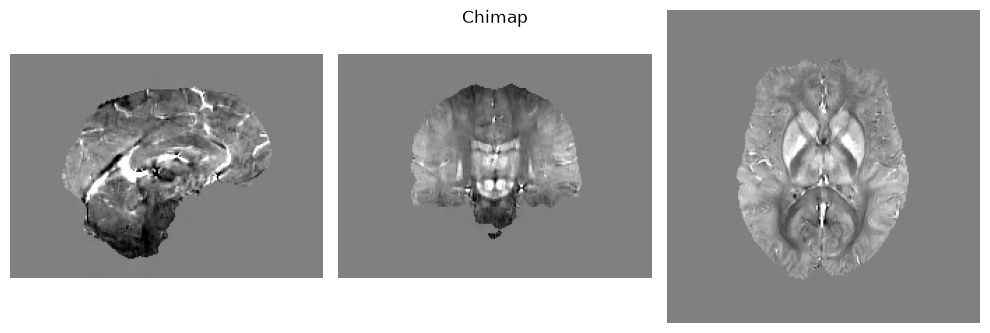
Segmentations
Segmentations are generated in both the QSM space and the T1-weighted space. Transformations are also made available.
show_nii(glob("bids/derivatives/qsmxt-*/sub-*/ses-*/anat/*qsm_dseg.nii*")[0], title="Segmentation", figsize=(10,8), cmap='Set3', vmin=0, vmax=96)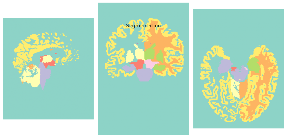
Analysis CSVs
CSV files have been exported containing susceptibility values in regions of interest for each subject.
Here we will load the CSVs, inspect the data and generate figures:
# import modules
import pandas as pd
import seaborn as sns
The raw CSV files use names from FreeSurfer as exported by FastSurfer. The full list of regions is available here.
pd.read_csv(glob("bids/derivatives/qsmxt-*-*/sub*/ses*/extra*/*.csv")[0])We will select a subset of these ROIs and give them more readable names:
# define regions of interest
# see https://github.com/QSMxT/QSMxT/blob/v8.1.1/qsmxt/aseg_labels.csv for a full list
rois = {
    "Thalamus" : [9, 10, 48, 49],
    "Pallidum" : [12, 13, 52, 53],
    "Caudate" : [11, 50],
    "Putamen" : [12, 51],
    "Brain stem" : [16],
    "CSF" : [24, 122, 257, 701],
    "White matter" : [2, 7, 41, 46, 177]
}
roi_names = { value: key for key in rois for value in rois[key] }
roi_ids = [value for roi in rois.values() for value in roi]
# load a reconstruction
qsm_img = nib.load(glob("bids/derivatives/qsmxt-*-*/sub*/ses*/anat*/*Chimap.nii*")[0])
seg_img = nib.load(glob("bids/derivatives/qsmxt-*-*/sub*/ses*/anat*/*space-qsm*dseg.nii*")[0])from nilearn.image import resample_to_img
# Resample the segmentation image to match the QSM image space
# Use 'nearest' interpolation to preserve the integer labels of the segmentation.
print("Resampling segmentation to match QSM dimensions...")
seg_resampled_img = resample_to_img(seg_img, qsm_img, interpolation='nearest')
print("Resampling complete.")Resampling segmentation to match QSM dimensions...
Resampling complete.
# Get data arrays
qsm = qsm_img.get_fdata()
seg = seg_resampled_img.get_fdata()
# Check shapes to confirm they match
print(f"Shape of QSM data: {qsm.shape}")
print(f"Shape of resampled segmentation data: {seg.shape}")
if qsm.shape != seg.shape:
raise ValueError("FATAL: Shapes not match after resampling. Check your input files.")Shape of QSM data: (224, 224, 160)
Shape of resampled segmentation data: (224, 224, 160)
# --- Flatten the arrays now that they have the same dimensions ---
qsm = qsm.flatten()
seg = seg.flatten()
# retain only the rois
qsm = qsm[np.isin(seg, roi_ids)]
seg = seg[np.isin(seg, roi_ids)]# convert to a dataframe for plotting purposes
seg = pd.Series(seg).map(roi_names)
data = pd.DataFrame({ 'qsm' : qsm, 'seg' : seg })# summarise data by region including the average and standard deviation
data.groupby('seg')['qsm'].agg(['mean', 'std']).sort_values('mean').round(decimals=3)medians = data.groupby('seg')['qsm'].median().sort_values()
order = medians.index# plot
fig, ax = plt.subplots(figsize=(5,4))
sns.boxplot(data=data, y='qsm', x='seg', fliersize=0, color='lightblue', order=order, ax=ax)
ax.set_xticks(range(len(ax.get_xticks()))) # Set tick positions explicitly
ax.set_xticklabels(ax.get_xticklabels(), ha='right', rotation=45)
ax.set_ylim(-0.2, 0.3)
ax.axhline(y=0, color='pink', linestyle='-', linewidth=1, zorder=-1)
ax.set_xlabel("Region of interest")
ax.set_ylabel("Susceptibility (ppm)")
ax.set_title("QSM")
plt.show()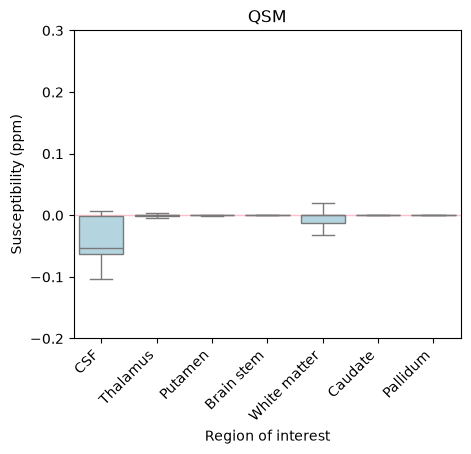
Dependencies in Jupyter/Python
Using the package watermark to document system environment and software versions used in this notebook, alongside the Neurodesktop version extracted from the
JUPYTER_IMAGEorNEURODESKTOP_VERSIONenvironment variables.
import os

%load_ext watermark

%watermark
%watermark --iversions

neurodesktop_version = (
    os.environ.get('JUPYTER_IMAGE', '').split(':')[-1] or
    os.environ.get('NEURODESKTOP_VERSION', 'unknown')
)

print(f"Neurodesktop version: {neurodesktop_version}")
Last updated: 2026-10-07T12:52:56.248169+00:00
Python implementation: CPython
Python version : 3.13.15
IPython version : 9.17.1
Compiler : GCC 15.3.0
OS : Linux
Release : 6.8.0-111-generic
Machine : x86_64
Processor : x86_64
CPU cores : 16
Architecture: 64bit
ipyniivue : 2.4.4
json : 2.0.9
matplotlib: 3.11.2
nibabel : 5.3.3
nilearn : 0.13.1
numpy : 2.3.5
pandas : 2.3.3
seaborn : 0.13.2
Neurodesktop version: 2026-10-05
- Stewart, A. W., Robinson, S. D., O’Brien, K., Jin, J., Widhalm, G., Hangel, G., Walls, A., Goodwin, J., Eckstein, K., Tourell, M., Morgan, C., Narayanan, A., Barth, M., & Bollmann, S. (2021). QSMxT: Robust masking and artifact reduction for quantitative susceptibility mapping. Magnetic Resonance in Medicine, 87(3), 1289–1300. 10.1002/mrm.29048
- Wang, Y., & Liu, T. (2014). Quantitative susceptibility mapping (QSM): Decoding <scp>MRI</scp> data for a tissue magnetic biomarker. Magnetic Resonance in Medicine, 73(1), 82–101. 10.1002/mrm.25358