EEG Analysis with MNE

Citation:¶

Tools included in this workflow¶

MNE-Python:

• Larson, E., Gramfort, A., Engemann, D. A., Leppakangas, J., Brodbeck, C., Jas, M., Brooks, T. L., Sassenhagen, J., McCloy, D., Luessi, M., King, J.-R., Höchenberger, R., Brunner, C., Goj, R., Favelier, G., van Vliet, M., Wronkiewicz, M., Rockhill, A., Appelhoff, S., … user27182. (2025). MNE-Python (v1.10.0). Zenodo. Larson et al. (2025)

• Alexandre Gramfort, Martin Luessi, Eric Larson, Denis A. Engemann, Daniel Strohmeier, Christian Brodbeck, Roman Goj, Mainak Jas, Teon Brooks, Lauri Parkkonen, and Matti S. Hämäläinen. MEG and EEG data analysis with MNE-Python. Frontiers in Neuroscience, 7(267):1–13, 2013. Gramfort (2013)

Tutorial this work is based on¶

• Analysing EEG Data with MNE by Angela Renton

Dataset¶

• Renton, A. (2022, April 11). Optimising the classification of feature-based attention in frequency-tagged electroencephalography data. Angela Renton (2021)

Install and import python libraries¶

Introduction¶

In this tutorial, we analyze EEG data from a visual attention task designed to evoke steady-state visual evoked potentials (SSVEPs). The dataset comes from an experiment in which participants viewed flickering fields of black and white dots, each assigned a different flicker frequency (6 Hz or 7.5 Hz, counterbalanced). Before each 15-second trial, participants were cued to attend to one color and detect brief bursts of coherent motion. On half the trials, both colors were presented concurrently (requiring selective attention), while on the other half, only the cued color was shown (mimicking complete attentional suppression). In our analysis, we focus on one participant and examine how attention modulates the frequency-tagged brain responses. After epoching and averaging trials by attended frequency, we use Fourier analysis to visualize how attention enhances SSVEP amplitude at the attended frequency.

Data download from OSF¶

Loading and preparing data¶

Begin by creating a pointer to the data:

The raw.info structure contains information about the dataset:

This dataset does not include a montage. We’ll use MNE’s built-in standard 10-20 montage to assign approximate electrode positions:

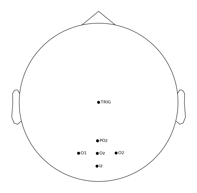
Next, let’s visualize the data.

In this notebook, the plot will be rendered as a static image (using Matplotlib as the 2D backend), so interactive features like scrolling through the time series are not available.

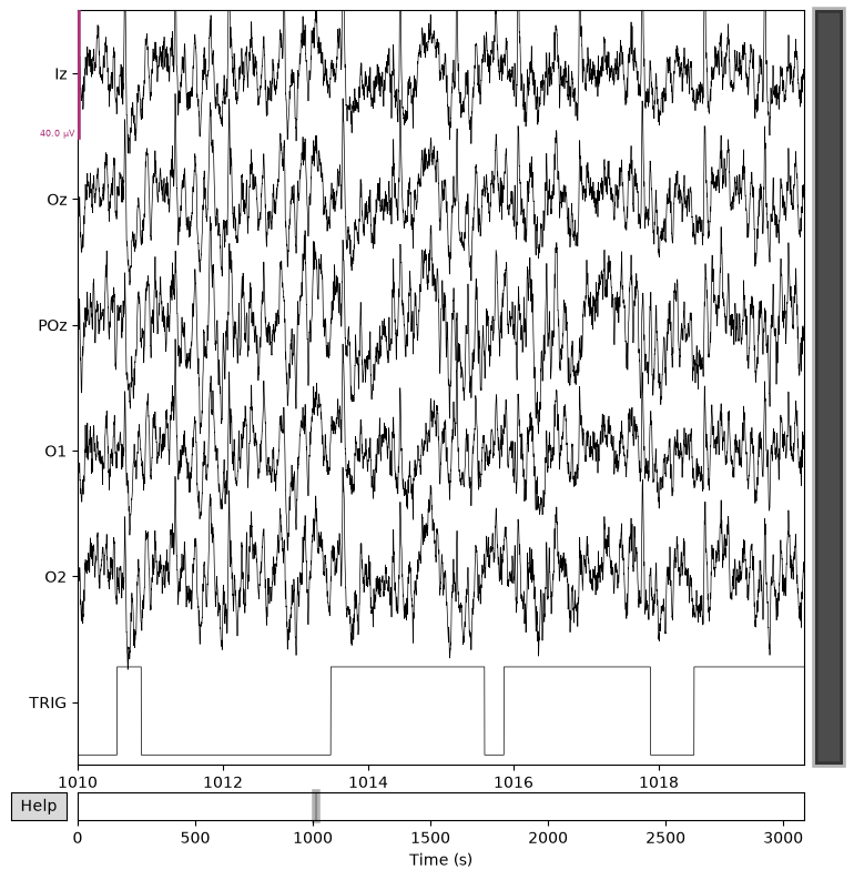
If, upon visual inspection, you decide to exclude one or more channels (e.g., due to noise or signal dropout), you can mark them as “bad” by adding them to raw.info['bads'].

For example, to mark channel ‘POz’ as bad:

This will ensure that the specified channel is ignored during subsequent preprocessing and analysis steps.

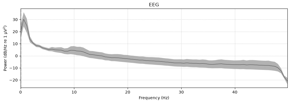
To visualize the frequency content of the continuous EEG data, use the compute_psd() method on the Raw object. The resulting Spectrum object’s plot() method will display the power spectral density (PSD). Since the data contains only EEG channels, the PSD will be shown for those channels.

To plot the average PSD across all EEG channels, use average=True and exclude any channels marked as bad.

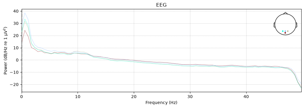
It is also possible to plot each EEG channel individually, with options for how the spectrum should be computed, color-coding the channels by location, and more.

For example, the following plot shows the PSD of the four selected sensors (specified via the picks parameter), with color-coding by spatial location enabled using the spatial_colors parameter. For full details, see the plot method documentation.

It is also possible to visualize spectral power estimates across sensors as scalp topographies using the Spectrum object’s plot_topomap() method. By default, this plots power in five frequency bands (δ, θ, α, β, γ), computes power based on magnetometer channels if available, and displays the estimates on a dB-like logarithmic scale.

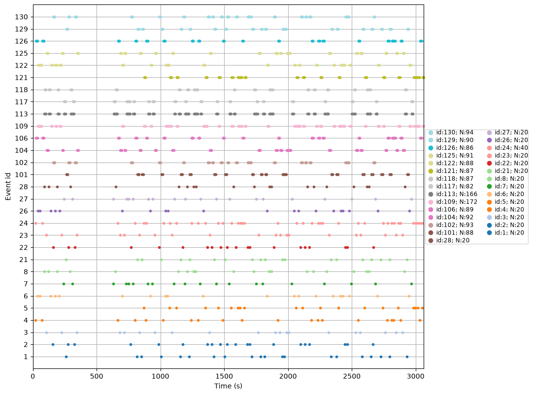
Extract Events¶

Next, we’ll extract events from the trigger channel. Since the trigger channel in this file is incorrectly scaled, we first correct the scaling before extracting the events.

Extract EEG Channels and Preprocess¶

Now that we’ve extracted events, we proceed with selecting the EEG channels and applying some simple preprocessing steps.

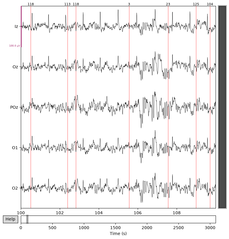
Epoching the Data¶

That’s looking good! We can even see hints of the frequency tagging. It’s about time to epoch our data.

We can average these epochs to form Event Related Potentials (ERPs):

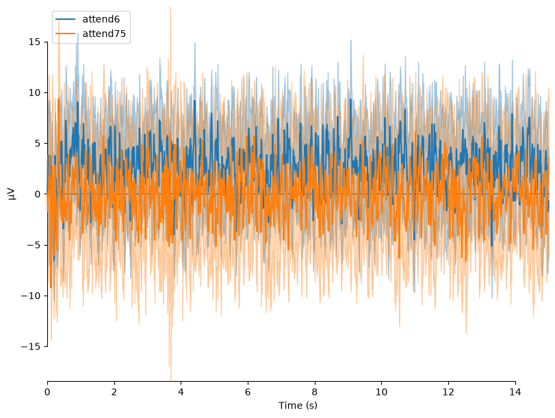
In this plot, we can see that the data are frequency tagged. While these data were collected, the participant was performing an attention task in which two visual stimuli were flickering at 6 Hz and 7.5 Hz respectively. On each trial the participant was cued to monitor one of these two stimuli for brief bursts of motion. From previous research, we expect that the steady-state visual evoked potential (SSVEP) should be larger at the attended frequency than the unattended frequency. First, we’ll examine how these frequency-tagged responses evolve over time, then quantify their overall strength. Let’s check if this is true.

FFT¶

Now let’s run a fast-fourier transform to evaluate how strongly our two tagged frequencies are represented in each condition.

Finally, let’s visualise the results.

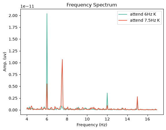
Exporting the data¶

Depending on what analyses you have planned, you may wish to extract the data from the mne format to a pandas or numpy array. Here’s an example of how we could run the same analysis using numpy and scipy. We’ll begin by exporting the averaged ERP data for each condition to a NumPy array, collapsing across EEG channels:

Next, we can use a Fast Fourier Transform (FFT) to transform the data from the time domain to the frequency domain. For this, we’ll need to import the FFT packages from scipy:

Now that we have our frequency transformed data, we can plot our two conditions to assess whether attention altered the SSVEP amplitudes:

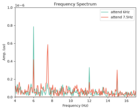
This plot shows that the SSVEPs were indeed modulated by attention in the direction we would expect!

Dependencies in Jupyter/Python¶

• Using the package watermark to document system environment and software versions used in this notebook, alongside the Neurodesktop version extracted from the JUPYTER_IMAGE or NEURODESKTOP_VERSION environment variables.