Analysing EEG Data with MNE

This tutorial was created by Angela Renton.

Github: @air2310

Getting started

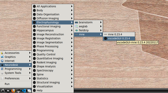
To begin, navigate to Neurodesk->Electrophysiology->mne->vscodeGUI 0.23.4 in the menu. This version of vscode has been installed in a software container together with the a conda environment containing MNE-python. Note that if you open any other version of vscode in Neurodesk, you will not be able to access the MNE conda environment.

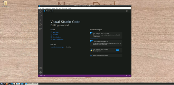
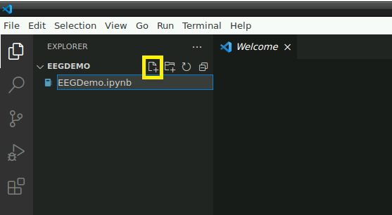
Open the folder: “/home/user/Desktop/storage” or a subfolder in which you would like to store this demo. In this folder, create a new file named “EEGDemo.ipynb” or something similar:

If this is your first time opening a Jupyter notebook on vscode in neurodesktop, you may see the following popup. If so, click “install” to install the vscode extensions for Jupyter.

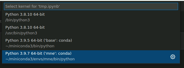
Select MNE python kernel

Next, we need to direct vscode to use the python kernel associated with MNE. In the top right corner of your empty jupyter notebook, click “Select Kernel”:

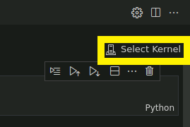
Then, select mne-0.23.4 from the dropdown menu, which should look something like this:

Activate the MNE conda environment in the terminal

Next, we’ll activate the same MNE environment in a terminal. From the top menu in vscode, select Terminal->New Terminal, or hit [Ctrl]+[Shift]+[`].

If this is your first time using vscode in this container, you may have to initialise conda by typing conda init bash in the bash terminal. After initialising bash, you will have to close and then reopen the terminal.

Once you have initialised conda, you can activate the MNE environment in the terminal:

conda activate mne-0.23.4

You should now see “(mne-0.23.4)” ahead of the current line in the terminal.

Download sample data

In the terminal (in which you have activated the MNE environment), input the following code to download some BIDS formatted sample EEG data:

Remember to update the path to the location you are storing this tutorial!

pip install osfclient
osf -p C689U fetch Data_sample.zip /neurodesktop-storage/EEGDEMO/Data_sample.zip
unzip Data_sample.zip 

This is a small dataset with only 5 EEG channels from a single participant. The participant is viewing a frequency tagged display and is cued to attend to dots tagged at one frequency or another (6 Hz, 7.5 Hz) for long, 15 s trials. To read more about the dataset, click here

Plotting settings

To make sure our plots retain their interactivity, set the following line at the top of your notebook:

%matplotlib qt

This will mean your figures pop out as individual, interactive plots that will allow you to explore the data, rather than as static, inline plots. You can switch “qt” to “inline” to switch back to default, inline plotting.

Loading and processing data

NOTE: MNE has many helpful tutorials which delve into data processing and analysis using MNE-python in much further detail. These can be found here

Begin by importing the necessary modules and creating a pointer to the data:

# Interactive plotting
%matplotlib qt

# Import modules
import os
import numpy as np
import mne

# Load data
sample_data_folder = '/neurodesktop-storage/EEGDemo/Data_sample'
sample_data_raw_file = os.path.join(sample_data_folder, 'sub-01', 'eeg',
                                    'sub-01_task-FeatAttnDec_eeg.vhdr')
raw = mne.io.read_raw_brainvision(sample_data_raw_file , preload=True)

the raw.info structure contains information about the dataset:

# Display data info
print(raw)
print(raw.info)

This data file did not include a montage. Lets create one using standard values for the electrodes we have:

# Create montage
montage = {'Iz':  [0, -110, -40],
            'Oz': [0, -105, -15],
            'POz': [0,   -100, 15],
            'O1': [-40, -106, -15],
            'O2':  [40, -106, -15],
 }

montageuse = mne.channels.make_dig_montage(ch_pos=montage, lpa=[-82.5, -19.2, -46], nasion=[0, 83.2, -38.3], rpa=[82.2, -19.2, -46]) # based on mne help file on setting 10-20 montage

Next, lets visualise the data.

raw.plot()

This should open an interactive window in which you can scroll through the data. See the MNE documentation for help on how to customise this plot.

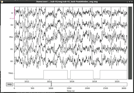
If, upon visual inspection, you decide to exclude one of the channels, you can specify this in raw.info[‘bads’] now. For example:

raw.info['bads'] = ['POz']

Next, we’ll extract our events. The trigger channel in this file is incorrectly scaled, so we’ll correct that before we extract our events:

# Correct trigger scaling
trigchan = raw.copy()
trigchan = trigchan.pick('TRIG')
trigchan._data = trigchan._data*1000000

# Extract events
events = mne.find_events(trigchan, stim_channel='TRIG', consecutive=True, initial_event=True, verbose=True)
print('Found %s events, first five:' % len(events))
print(events[:5])

# Plot events
mne.viz.plot_events(events, raw.info['sfreq'], raw.first_samp)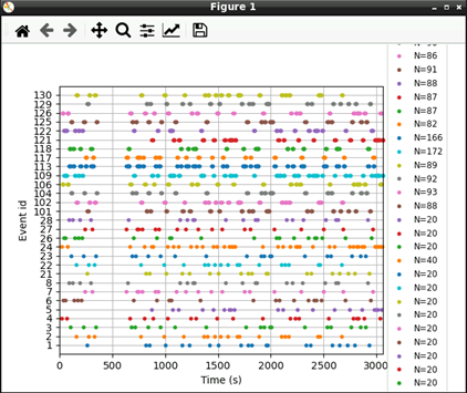

Now that we’ve extracted our events, we can extract our EEG channels and do some simple pre-processing:

# select
eeg_data = raw.copy().pick_types(eeg=True, exclude=['TRIG'])

# Set montage
eeg_data.info.set_montage(montageuse)

# Interpolate
eeg_data_interp = eeg_data.copy().interpolate_bads(reset_bads=True) 

# Filter Data
eeg_data_interp.filter(l_freq=1, h_freq=45, h_trans_bandwidth=0.1)

Let’s visualise our data again now that it’s cleaner:

#plot results again, this time with some events and scaling. 
eeg_data_interp.plot(events=events, duration=10.0, scalings=dict(eeg=0.00005), color='k', event_color='r')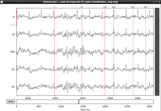

That’s looking good! We can even see hints of the frequency tagging. It’s about time to epoch our data.

# Epoch to events of interest
event_id = {'attend 6Hz K': 23, 'attend 7.5Hz K':  27}  

# Extract 15 s epochs relative to events, baseline correct, linear detrend, and reject 
# epochs where eeg amplitude is > 400
epochs = mne.Epochs(eeg_data_interp, events, event_id=event_id, tmin=0,
                    tmax=15, baseline=(0, 0), reject=dict(eeg=0.000400), detrend=1)  

# Drop bad trials
epochs.drop_bad()

We can average these epochs to form Event Related Potentials (ERPs):

# Average erpochs to form ERPs
attend6 = epochs['attend 6Hz K'].average()
attend75 = epochs['attend 7.5Hz K'].average()

# Plot ERPs
evokeds = dict(attend6=list(epochs['attend 6Hz K'].iter_evoked()),
               attend75=list(epochs['attend 7.5Hz K'].iter_evoked()))
mne.viz.plot_compare_evokeds(evokeds, combine='mean')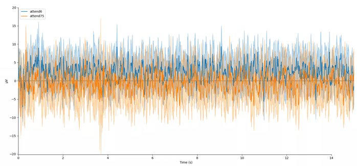

In this plot, we can see that the data are frequency tagged. While these data were collected, the participant was performing an attention task in which two visual stimuli were flickering at 6 Hz and 7.5 Hz respectively. On each trial the participant was cued to monitor one of these two stimuli for brief bursts of motion. From previous research, we expect that the steady-state visual evoked potential (SSVEP) should be larger at the attended frequency than the unattended frequency. Lets check if this is true.

We’ll begin by exporting our epoched EEG data to a numpy array

# Preallocate
n_samples = attend6.data.shape[1]
sampling_freq = 1200 # sampling frequency
epochs_np = np.empty((n_samples, 2) )

# Get data - averaging across EEG channels
epochs_np[:,0] = attend6.data.mean(axis=0)
epochs_np[:,1] = attend75.data.mean(axis=0)

Next, we can use a Fast Fourier Transform (FFT) to transform the data from the time domain to the frequency domain. For this, we’ll need to import the FFT packages from scipy:

from scipy.fft import fft, fftfreq, fftshift

# Get FFT
fftdat = np.abs(fft(epochs_np, axis=0)) / n_samples
freq = fftfreq(n_samples, d=1 / sampling_freq)  # get frequency bins

Now that we have our frequency transformed data, we can plot our two conditions to assess whether attention altered the SSVEP amplitudes:

import matplotlib.pyplot as plt

fig,ax = plt.subplots(1, 1)

ax.plot(freq, fftdat[:,0], '-', label='attend 6Hz', color=[78 / 255, 185 / 255, 159 / 255])  
ax.plot(freq, fftdat[:,1], '-', label='attend 7.5Hz', color=[236 / 255, 85 / 255, 58 / 255])  
ax.set_xlim(4, 17)
ax.set_ylim(0, 1e-6)
ax.set_title('Frequency Spectrum')
ax.legend()

This plot shows that the SSVEPs were indeed modulated by attention in the direction we would expect! Congratulations! You’ve run your first analysis of EEG data in neurodesktop.